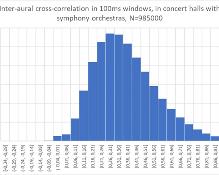
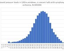
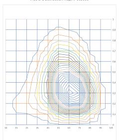
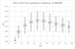
Binaural Project status update after 11 years of recording and analysis.

Statistical distribution of listening levels and Inter-Aural Cross-Correlation (IACC) from 98500 seconds (27 hours and 22 min) of symphonic music in concert halls world-wide.

Distributions of nearly one million events, each lasting 1/10 s. Passband filter 400-2500Hz. Analysis window length 100ms.

The most frequent IACC is 0.3 (+/-0.05), occuring in 22% of the music.

The most frequent listening level is 64-67dB, occuring in 8% of the music, and events at this level also display the biggest variation in IACC, as can be seen in the two-dimensional distribution chart (Figure 3). High values of IACC indicates strong localization in soloist parts, woodwinds in particular, naturally occuring at medium listening levels.

The typical 100ms-event is 50dB with IACC=0.3

Higher listening levels with lower IACC occur in the more powerful tutti parts with an impression of source broadening. Strong solo parts are rare.
Background noise and reverb tails in the music are typically omni-directional with low IACC, and they occur naturally at low levels.

Figure 1 (above, left) IACC Histogram after 98500 seconds of symphonic music listening
Figure 2 (above, right) Listening levels histogram (dB) after 98500 seconds of symphonic music

Figure 3 (above, left) Two-dimensional distribution over IACC and listening levels (dB) after 98500 seconds of symphonic music;
Maximum likelihood: IACC=0.30 at 65dB in 6.3% of the time.
Figure 4 (above, right) Statistics of IACC at various listening levels (dB) after 98500 seconds of symphonic music

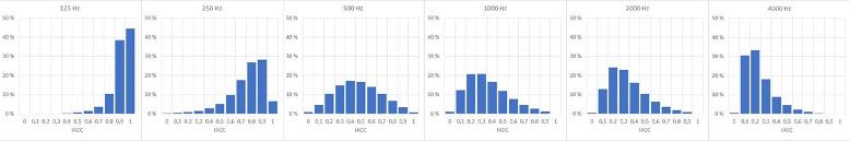
Figure 5 Histograms of IACC in octave bands 125-4000Hz after 93.000 seconds of symphonic music

Figure 6 Histograms of listening levels (dB), in octave bands 125-4000Hz, after 93.000 seconds of symphonic music

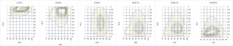
Figure 7 Two-dimensional distribution over IACC and listening levels (dB) in octave bands 125-4000Hz  after 93.000 seconds of symphonic music

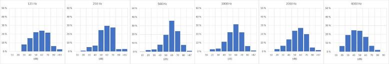
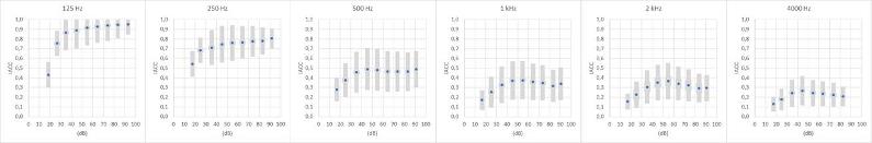
Figure 8 Statistics of IACC in octave bands 125-4000Hz at various listening levels (dB) after 93.000 seconds of symphonic music

Binaural Dynamics in Broadband IACC
To calculate the single-value IACC in the binaural signal, a filter with passband 400-2500Hz is used (-10dB points at 200Hz and 2700Hz)

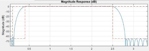
Figure 9 Broadband Filter used in the current binaural signal analysis

When analyzing sequences of 100ms windows, each window is sufficiently long to allow for its content to be perceiveable.

In a window containing the onset of a musical note in an insturment, direct sound from that instrument would increase, causing two simultaneous effects at the listeners ears: 1) A level increase, 2) an increase in IACC because direct sound add a similar signal to both ears.

Opposite, the offset of a note would cause both level and IACC to drop, because direct sound disappears, leaving a reverberant decay.

Music is not just pure onsets and offsets, but the coinciding increase and decrease even happens with expressive dynamical playing style, crescendi and decrescendi, or due to tremolo or other vibrato effects.

From our huge amount of data we see that typically, increments and decrements in Level and IACC coincide in 60% of the binaural signals in live symphonic music. Why not 100% and what happens in the 40% other mini-events in music? Well, there are numerous of complex events, like fluctuations in modes, fluctuations from interfering tones, fluctuating directivity or directive instruments that are moving. superposition from many instruments, strong lateral early reflections, and so on, causing IACC to decrease while level increase, and vice versa.

Visualizations of level and binaural dinamics

In the following diagrams, the more vigorous the binaural dynamics, the fluffyer the curves.

Definitions:

Differential, a change in metric value from one window to the next, e.g. DIACC = –0.06 if a window is 0.53 and the previous is 0.59

Increment, a rise in metric value from one window to the next in a sequence of windows, i.e. DIACC >0.0, or DL>0dB

Decrement, a reduction in metric value from one window to the next, i.e. DIACC <0.0, or DL<0dB

Coherent Differentials, in two succeeding windows where DIACC >0.0 AND  DL>0dB, or where DIACC <0.0 AND  DL<0dB

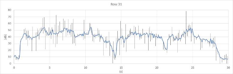
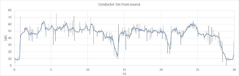
Figure 10 Level profile and IACC increments from oboe solo, see text below. Link to the sound  (use earphones) opens in separate window.

In Figure 10 the solid curve is the level in dB from an oboe solo reproduced with a loudspeaker on the empty stage in Oslo Concert Hall, as recorded at Row 31, over a 30s period (Horizontal axis). The feather-like bars indicate events where an increase in level is accompanied by an increase in IACC, and opposite. The heigth of the curves are 40 times the changes in IACC values, e.g. an increase from  0.40 to 0.45 would be indicated with a bar of height 40x0.05 = 20, which in the diagram would be two gridlines.

Interpretation: A bar pointing upwards would be perceived as an increase in IACC and thus a more point-like or narrow sound image, while a downward bar would indicate a wider sound image. 3 musical phrases can be seen, with brief pauses at 14 and 22 second.

On average, there are 6-7 bars per second so obviously they are not all onsets and offsets, but a combinatiuon of musical expressions and fluctuations in the transmission from source to receiver. After the last note, at 28 s, the reverberant decay has consistently decreasing IACC, caused by the omni-directional reverberant sound field.

In this 30s example consisting of 300 windows, the statistics of the coherent IACC-differentials (in this case 66% of the signal) described above are
-0.01±0.25 in terms of average and standard deviation. The larger the standard deviation, the greater the dynamics of the binaural sound image, i.e. the bigger the span between narrow events and wide events. Average of the whole 30s signal is IACC=0.45.

The complex binaural signal from symphonic music at listeners ears have IACC-differentials on average 0.00 and standard deviation in the range of ±0.15 to ±0.20. So far, no significant differerences between halls as far as IACC-differentials have been observed.

In the excact seat in Row 31 in the example above, the average IACC through the 6 movements of Mahler III were in the range of 0.34 to 0.38, while coherent differentials (in 59% of all 100ms windows) had a standard deviation of ±0.17 to ±0.19.

The closer to the instrument the listener comes, the more will direct sound dominate and the higher will average IACC be. Figure 11 shows the level and IACC-differentials at conductors position at 5m distance from the excact same source as in the example above, Row 31, in Figure 10.

Statistics over the 30 seconds:  Average IACC=0.70.  Coherent differentials (66% of all windows) average and standard deviation: –0.01 ±0.19.  As expected IACC average is higher at conductors position than at Row 31, while standard deviation of differentials is smaller, down from ±0.25 to ±0.19. The perceived difference at conductors position would be a clearer, narrower sound image with less powerful binaural dynamics, less audible envelopment.

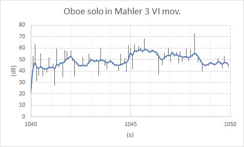
   Figure 11, same music and source as in Figure 10, but listening at conductors position at 5m distance. Link to the sound .

The next example, Figure 12, is an oboe solo in a live performance of Mahler’s 3rd Symphony — from the breaking part after 4-5 minutes of pure string orchestra in the beginning of the 6th movement. The listening position is the excact same chair in Row 31 as the example in Figure 10.  IACC=0.48 and differentials are DIACC =  0.01 ±0.19. Note that in this live case, average IACC is 0.03 higher, while the dynamic binaural deviation is  significantly smaller, with ±0.19 instead of ±0.25, which is most likely due to the strings smoothing out the sound image somewhat.

Figure 12 Oboe solo, live performance of Mahler 3rd, see teaxt. Link to the sound .

		IACC average	BSD	Coherent Differentials Frequency	dB
BPh	T3	0,33	0,17	56 %	56
BSH	Brahms violin concert	0,35	0,18	59 %	52
SKH	T4	0,32	0,17	59 %	74
SKH	T4 II oboe	0,45	0,22		64
SKH	t4 II cello section	0,19	0,18		69
COH	T4	0,38	0,18	59 %	74
COH	T4 II oboe	0,48	0,20		58
COH	t4 II cello section	0,47	0,20		69
ACG	Mussorgskij Pictures	0,38	0,19	60 %	74
OKH	Mahler 3	0,36	0,18	59 %	65
OKH	Mahler 3 VI oboe	0,48	0,19		59
OKH	Mahler 3 VI strings	0,39	0,20		54
OKH	oboe solo loudspeaker	0,45	0,25	66 %	48
LaScala	Mahler 2	0,42	0,18	59 %	55

Figure 13 Examples of data from music in 7 different halls. BSD is binaural, standard deviation, see text for explanations.

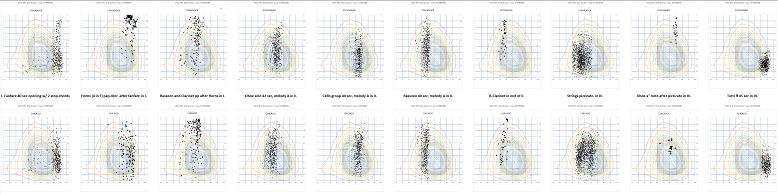
IACC and Level maps from two concert halls while listening to the same music

The diagrams below are plots of IACC and Levels (dB) over the statistical map in Figure 3, measured while listening to Tchaikovsky’s 4th Symphony.   Upper row is from Stavanger Konserthus, lower row is from Chicago Orchestra Hall. The 10 pairs of plots are 10 parts through the 4 movements of the symphony, chronologically ordered from left to right.

I. Fanfare ff

I. Horns X4 in F

Bassoon and Clarinet pp

II. Oboe solo 42 sec, melody A

II. Cello group 40s melody A

II. Bassoon 40 sec, melody A

II. B-Clarinet end of movement

III. Strings pizzicato theme

III. Oboe single a'' note

VI: Tutti ff 45 sec

Figure 14, IACC and Levels (dB) in two concert halls, see text above.

Variation in the IACC-data, categories and  statistical populations

Significant differences between halls, in average IACC from one and the same symphony, has been observed. 

However, the biggest variation in IACC is due to variation in the music itself. One example can be seen in two of the diagrams, where music of different loudness form different "populations" of IACC.

Oboe solo, string section and tutti appear to be other examples of different populations, or categories if you like.

References:

The Binaural Signal From a Symphony Orchestra 
Live listening vs Headphone listening

Se also links on top of page

Page created 26.02.2020

Latest change 15.02.2023

Binaural Project sub-pages

Binaural Project links

Binaural Project Startpage

Measurements of IACC during music performance in concert halls 01.02.2017

BRIR buildup

ISMRA presentation 11.09.2016, ASA-Boston-2017-presentation 29.06.2017

IACC (BRIR) data from concert halls

ICSV24 London paper 2017

Live listening vs Headphone listening

The Binaural Signal From a Symphony Orchestra

Result, status and statistics