
|
Live listening vs headphone listening |
|
Abstract Localization, Source Broadening and Envelopment are among the listening aspects necessary to achieve excitement and engagement when listening to a live classical music performance. A playback of a binaural recording in headphones can quite accurately reproduce the sonic impression from the concert. In contrast, common stereo recordings techniques are very different from those used for binaural recordings. Newer generations seem to enjoy all kinds of recorded and streamed music in headphones. Can a good recording provide binaural signal qualities equivalent to those of a good live event? For newer recordings the answer seems to be no. Older recordings seems to be more similar to live, as far as the IACC-comparisons in this investigation can tell. However, a full similarity test would need more detailed investigation. Considering the nature of common practical recording techniques, similarity with live listening is not possible. Redirect to video presentation and slides in PDF by clicking here |
|
1. Introduction
Localization, Source Broadening and Envelopment are among the listening aspects necessary to achieve excitement and engagement when listening to a live classical music performance. These spatial, perceptive aspects are again related to certain features in the binaural signal arriving at the listeners ears.
A playback of a binaural recording[1] in headphones can quite accurately reproduce the sonic impression from the concert. In contrast, common stereo recordings techniques are very different from those used for binaural recordings. Newer generations seem to enjoy all kinds of recorded and streamed music in headphones. This paper will compare features of the binaural signals from live classical performance with high-quality stereo recording of the same piece of music when listened to in headphones. Can a good recording provide binaural signal qualities equivalent to those of a good live event, or does the classical concert venue have something unique and irreplaceable to offer newer generations? What difference does room acoustics make to binaural signal in facilitating a musical experience? These are key questions to be addressed in this paper.
Since 2011, this author has run the Binaural Project, aiming to explore the nature of the binaural signal through measurements in live music performances with symphony orchestras. The basics of the projects are described on the project’s web page[2]. In this paper, the problem complex introduced above is approached by to the question: What differences and similarities between live concert listening and headphone listening can be seen in the binaural signals presented to the ears in the two cases?
Specifically: Would the difference between the sound in one concert hall and the sound from a record be bigger or smaller than between the two concert halls? Here, “a record” in 2020-terms would mean a wide range of available recording and reproduction formats, from traditional recording to modern streaming by YouTube, Spotify, etc. To address the specific question, the following method was chosen. |
|
2. Method
2.1 Data and formats A direct method was chosen. Binaural signals from live music listening was compared with the exact same pieces of music, although played by different orchestras, reproduced via different media and played back in earphones. The binaural signal measurements were made with tiny microphones in the ear canal according to the procedure in the Binaural Project description. This technique allows the measurement objects, i.e the signal input reaching the entrance of the ear canal of the listener, to be changed without changes in the measurement signal chain. In short, the differences heard are the differences measured. Thus, any difference in perceived sound has the same cause as any difference in the binaural signal reaching the recording device. All the binaural signals forming the raw data in the investigation reported in this paper have been recorded with the one and same H2 Zoom wave-recorder, at 16-bit rate, 128 bit/s, sampling frequency 44.1kHz, and stored in the common wave-format with file extension *.wav.
2.2 Inter-aural cross-correlation IACC
Inter-aural cross-correlation IACC is a common quantity in research and findings in binaural hearing, as well as in the binaural cues and parameters in concert hall acoustics. Thus, it was natural base the investigations in the Binaural Project on IACC. The algorithm used to convert the binaural signal pair from the left and right ears, to a sequence of IACC-values can in short be described as follows
· Filtering, from each signal producing a set of 6 signals, one for each octave band 125Hz to 4kHz · Dividing the signal into a sequence of 100ms periods, each with 441 samples · From each 100ms period and each octave band compute the normalized cross-correlation function IACCF(i) for the 47 different lags from i=-23 samples lag*, to i=+23 samples lead, taking values in the range [-1.0,1.0] · Inter-aural coherence IC=IACCF(0), is the special case i=0, with neither lead or lag, which would be the inter-aural cross-correlation from sound arriving from a source up front, i.e. a source in the median plane; in an-echoic conditions a source in the median plane would ideally produce IC=1.0 · In each 100ms period above, the highest value of IACCF(i) returned from calculations with the 47 different lags, define each term in the IACC(t) sequence in each octave band IACC(t)=max {IACCF(i)}, where t belongs to any sequence t=t0+n·0.1s, where n=0,1,2,….
Note that the normalization of the IACCF cancels out any differences between left and right ear as to biased SPL or gain differences in the measurement chain.
*(23 samples lag is 0.52 ms, the delay from a 17.7cm detour around the head. In common binaural hearing models, a signal arriving from left would arrive at the right ear with approximately 23 samples lag relative to signal arriving at the left ear. With i the number of sample lags, t=i/44.1kHz, IACC(i) converts to the common form IACC(t).
2.3 Examples of IACC
In an-echoic conditions a sound source would cause the inter-aural cross-correlation function to take the value IACCF(i)≈1.0 for one of the sample-lags i, depending on the direction of arrival. Our IACC(t) is not intended to tell us in what direction the source is, it just tells us how strong cross-correlation is in the direction where the highest value is detected.
In reverberant conditions, or in any presence of noise or other sound that is not correlated with the direct sound, we would observe lower values than IACC(t)=1.0. How low depends on frequency, for the following reasons.
When sound arrives from a source at one side of the head, sound would need to take a longer path around the head to the ear on the far side ear than to ear on the near side. From the mid-frequency (MF) range, octaves 500 and 1000Hz, und upwards, the extra path length would cause a phase difference between the two ears. In these octaves, even a single sample lag could cause a noticeable difference in the IACCF, and in common hearing models, phase differences provide the dominant ques for sound source detection and the listener aspect of Localization. Above 1500Hz, our hearing would also take cues from the inter-aural level-differences (ILD) caused by the sound shadow on the far side of the head when sound arrives from off-axis.
In the low-frequency (LF) region, towards zero frequency, the IACC(t) would approach 1 regardless of the direction of the source, since the human head is too small, and the wavelengths of the acoustic signal too long, for there to be a difference between the signals at the two ears. Examples: Figure 1; In diffuse conditions in 125Hz we observe average values around IACCL=0.90 in the late reverberant decay, i.e. after 80ms. In the early part of the binaural impulse response, we have statistically IACCE=0.93. The significance of IACC in the LF-region is unclear, and in this paper the observations in LF will only be briefly mentioned. In the following, the octaves 500-4k will be emphasized.
Fig 1 |
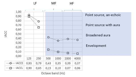
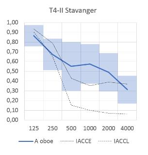
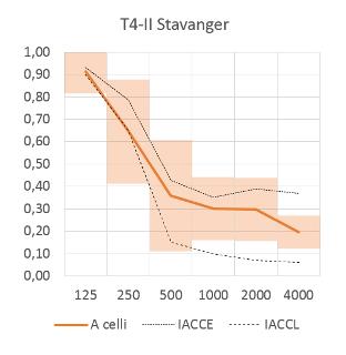
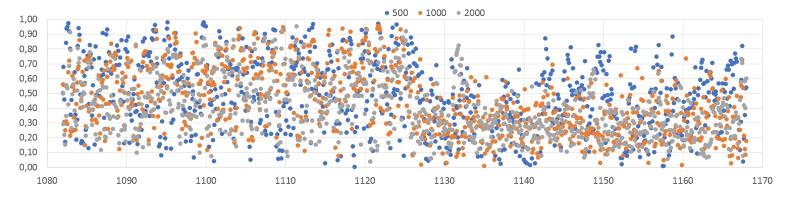
2.4 Interpretations of IACC in reverberant conditions, 500Hz – 4kHz octave bandsWhen reverberant sound is weak, i.e. with direct sound dominating and direct-to-reverberant ratio is d/r>>1, IACC would take values close to 1. The point source would be perceived as point-like. In the limit where d/r=1, if the reverberant sound is relatively diffuse, IACC would be close to 0.7. A point source would be perceived as moderately broader than at IACC=1. Some listeners would describe the broadening as an aura or halo around the point source. If the reverberant sound is dominated by lateral reflections, the value would be lower than 0.7, and higher than 0.7 if vertical reflections dominate. The so-called aura would be perceived bigger for lower values of IACC. As d/r decreases below d/r=1, e.g. if the listener moves away from the source, IACC would decrease. The perceived aura would grow bigger. In the average concert hall, IACC from the first 80ms of an impulse response, IACCE, would be close to 0.4 in the octave bands 500-4k, Figure 1. If lateral reflections are dominating over vertical reflections, IACC would take lower values than if vertical reflections dominate over lateral reflections. When sound comes from a group of instruments distributed over the stage, IACC would naturally take lower values than when sound comes from a single instrument. Consistently, like with source broadening of a single instrument, a broader source would come with lower IACC than a source that actually is perceived as a point source. When d/r approach zero, IACC could approach the values seen in the late part of the impulse response in the classical, rectangular concert halls, like those in Vienna, Amsterdam and Boston, where IACCL in the range 0.15 in 500Hz down to 0.06 in 4kHz, the lower curve in Figure 1. In this low limit, the sound image is diffuse, without any frontal emphasize. Here, it is important to keep in mind that during a music performance, IACC(t) hardly stabilizes to a constant value, but instead fluctuates heavily around a floating average. When this floating average is advantageous, fluctuations would cause ques of perception that fluctuates in the span between localization and envelopment. Example 1: Figure 2, left part. During an oboe-solo in a symphony orchestra performance in a good concert hall, IACC could fluctuate around an average of 0.60, with brief instants below zero and up to 0.98, upper quartile around 0.85 and lower quartile around 0.40. This means that 25% of the instants have values in the range 0.85 to 0.98, with strong cues of Localization. Equally, 25% of the instants have values in the range 0.0 to 0.40. More than 80 dots below 0.20 can be counted, more than twice per second, providing strong cues of Envelopment. The mediate range between 0.40 and 0.85 would have ques of Source Broadening. Example 2, Figure 2 right part. When the cello section repeats the melody of the oboe solo, a more compact distribution around a lower average is observed, with a naturally broader sound image from a distributed, broader source like the cello section actually is. Still, as many as 40 dots (500Hz) above 0.70 can be counted between 1140 and 1170s, on average one per second, being brief instants of point-like localization, as if the individual instruments have fluctuating directivity. In optical analogy, the cellos are sparkling.
Figure 2: Lower diagram, IACC(t) in 500, 1000 and 2000Hz plotted over time between 1080s and 1170s during Tchaikovsky’s 4th Symphony in Stavanger Concert Hall, beginning of 2nd movement Andantino. 1080s to 1125s is an oboe solo, while 1125s to 1170 is the same melody repeated by the cello section; Upper diagrams are statistics from the same parts, oboe to the left, and cello section to the right, solid curves are average IACC, shaded area span between lower and upper quartiles (25p-75p), and dotted curves the references for IACCE and IACCL. |
2.5 Comparison methodDifferences and similarities between the various material presented below, are measured by comparing statistics from the IACC(t) data of the material. The music is divided into parts after musical category or because they are observed to have different statistics. Examples of such categories are musical categories like solo parts, string section parts, tutti parts, parts with brass, strong, soft or medium strong parts, melodic themes, and so on. Some comparisons would be to see to what degree a transition from one part to the next happens with the same change in IACC in when comparing to versions of the same music. In particular, we would like to know whether a solo part has higher IACC than a full string section part in a recording, like it does in a live performance. For this purpose, the second movement of Tchaikovsky, T4-II for short, is divided into 36 parts, T4-IV in 20 parts, and Prokofiev’s violin concert in 51 parts. Spectrograms are useful in detecting transitions between parts with significant differences, like the one in Figure 3. IACC-profiles of each case from various material was computed. Examples of IACC-profiles of T4-II, is presented in Figure 4. In the results section below, systematic comparisons of all the investigated material, in all octave bands are carried out with a regular correlation algorithm. In live listening, the fluctuating IACC-values typically exhibit gaussian distribution. In recording, d/r may be chosen so high that the upper tail in the gaussian distribution is forced to be truncated, which would mean a significantly different perception of music than the live listening case. Some results call for more detailed investigation, and thus ad-hoc analysis methods.
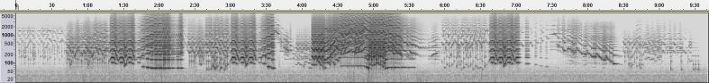
Figure 3 Spectrogram of T4-II recorded with Oslo Philharmonic in 1984; Arrows indicate some of the transtions of interest between parts with significant differences; The first arrow indicate the transition between the oboe solo and the repetition in cellos in Figure 2
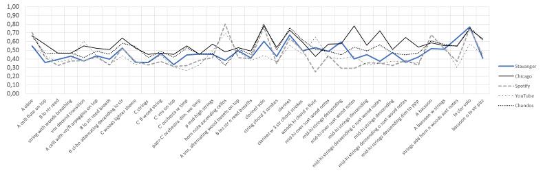
Figure 4: IACC in the 500Hz band, averages from 36 parts of the 2nd movement of Tchaikovsky’s 4th Symphony, for comparison between live listening in Stavanger and Chicago, Spotify listening, YouTube listening and listening to a wave-file from a traditional recording (Chandos). Letters A, B and C are arbitrary notations by the author, to identify different themes (melodies). The leftmost parts “A oboe” and “A celli” correspond to the exampes in Figure 2. |
2.7 Data materialTwo live concerts with Tchaikovsky’s 4th symphony (T4), performed by two different orchestras in two different countries, in two different years offered a starting point. From these it is possible to get an idea of differences and similarities that can occur within from one concert to another. A selection of different available down-loadable recordings of T4 was chosen from the top hits in google, when searching the expression “Tchaikovsky’s 4th symphony”, one bought from Chandos, one free-version from Naxos, one top hit version from YouTube, and one version from Spotify. A list of the data material in given in Table 1.
Table 1 List over the data used in the current investigation
|
3 ResultsThis section presents the results from the investigation, according to the methods described above. Average of IACC(t) in Figure 5. Basic differences and similarities are also evaluated by the correlation between IACC-profiles of each listening cases in Table 2 , by the histograms Figure 5, and the IACC-dynamics ratio diagrams in Figure 6 and Figure 7.
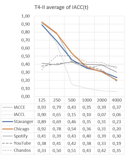
Figure 5 a (above): Average of IACC(t) over octave bands 125 to 4000Hz, Tchaikovsky 4th symphony 2nd movement.
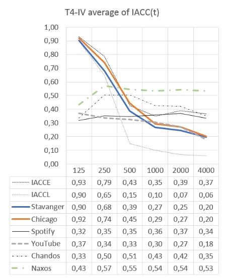
Figure 5 b (above): Average of IACC(t) over octave bands 125 to 4000Hz, Tchaikovsky 4th symphony 4th movement.
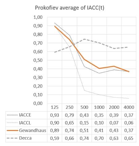
Figure 5 c (above): Average of IACC(t) over octave bands 125 to 4000Hz, Prokofiev’s violin concert. |
|
|

|
Histograms of the Prokofiev violin concert reveal one of the critical differences between the live listening and the recording, both with violin soloist star Janine Jansen, Figure 5.
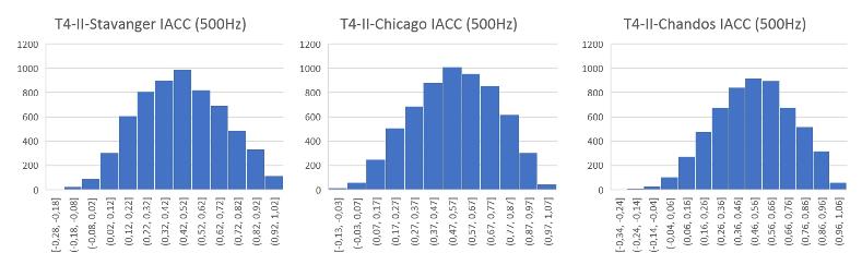
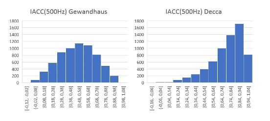
Figure 6 Histograms of IACC in the 500Hz octave; Upper row is Tchaikovsky’s 4th Symphony, 2nd movement, where Stavanger and Chicago are live listening, and the rightmost “Chandos” is headphone listening to a recording from 1984 with Oslo Philharmonic Orchestra in Oslo Concert hall, all of which exhibit gaussian bell-shapes with slighly different skews. Lower two diagrams are Prokofiev’s violin concert, where the leftmost, Gewandhaus, is live listening, exhibiting a bell-shape similar to those in the upper row. The rightmost, Decca, is a recording with the same violinist, exhibiting a truncated bell-shape in the high end of the IACC-scale. |
|
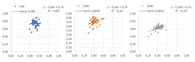
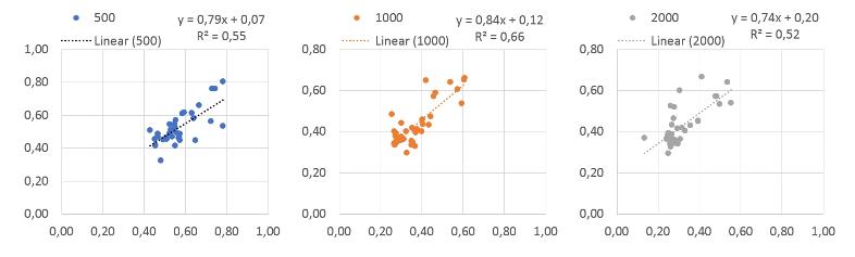
Figure 7: IACC dynamics in Prokofiev; IACC in 51 parts in live listening in Gewandhaus (horizontal axis) plotted against IACC in the same parts while listening to a Decca recording with the same violin soloist. R2, and the factor a in y=a*x indicate the similarity between IACC dynamics in live listening and IACC dynamics in the recording. R2 =1 and a =1 would indicate full similarity, while R2 =0 and a =0 would indicate no similarity. |
|
Figure 8: IACC dynamics in T4-II; IACC in 36 parts in live listening in Chicago (horizontal axis) plotted against IACC in the same parts while listening to tha Chandos recording. High values of R2 and the y/x ratio indicate high degree of similarity in IACC between the two cases. When IACC increases in Chicago it would increase in the Chandros record. E.g., this means that in parts where Localization is sharp in Chicago would also have sharp Localization in Chandros. Conversely, when Source Broadening increases in Chicago, it will increase in Chandros. |
4 Comments and conclusionsVarying degree of similarity between live listening and listening to records in headphones is seen in the results. In the Tchaikovsky cases the similarity between live listening in Chicago and headphone listening to Chandos (OFO 1984) is bigger than the similarity between live listening in Chicago and live listening in Stavanger. The Naxos recording from 2005 is an example of the opposite, similarity with live listening is poor. The poorest similarity in the material is seen between the Decca record of Prokofiev with soloist Janine Jansen in 2012 and the live listening with the same music and soloist in Leipzig Gewandhaus, row K a year or two before the recording. In general the similarities between live and recordings are bigger in the fourth movement of Tchaikovsky than in the second movement. This author explains this by the second movement having a bigger dynamic range in the IACC, making it more difficult to emulate with common recording techniques. The diagrams in Figure 6 demonstrates why an excessive use of direct sound from close microphones creates overall high IACC-values, making it impossible to recreate the dynamics of IACC, so important to the live listening experience. This problem also manifests in the truncated bell-shape in the histogram in Figure 5. Some recording engineers have suggested that there is a trend towards more d/r ratio in recordings, inevitably causing problems with higher IACC and loss of IACC dynamics. In this investigation at least, this seems to be the case. The older recordings are found to offer headphone listening more similar to live listening than the newer ones. The perceptive effect of un-natural low and random-like IACC in 125Hz and 250Hz like those seen in record listening in this material, while not in live listening, is unclear. This investigation has been limited to use of IACC, which indeed carries information of how the degree an instant source is point-like or broad, but unlike the IACCF it ignores in what direction the source is. Any mismatch between ITD and ILD that would potentially affect the listening experience will not be included in the assessment of similarity in this paper. In common recording techniques, so-called panning (ILD control in intensity stereo) could e.g. localize the high frequencies of the violin section to the left, while their fundamental frequency could be anywhere in the sound image, since the latter is detected by ITD and its phase-differences. In a more complete assessment of similarities in future work, these issues will need to be investigated. |
5 Discussion: What to expect from recorded orchestra musicWhile the three listener aspects of Localization, Source Broadening and Envelopment are appreciated by recording engineers, the challenges in combining them all in one and the same recording are well known. Ideally, a binaural recording, e.g. with a dummy head in a good audience position would preserve all three aspects. It would be a pure reproduction of the signal that reaches the ears of a listener at the actual position. However, a range of practical issues inevitably lead to a series of compromises. For one, the recorded sound would depend a lot on the acoustics of the recording space, and this is not always wanted. Moving the microphone position closer to the orchestra could reduce the relative influence of the room acoustics and allow freedom to add artificial reverb on demand in the post-processing. But the microphones would need to fly above the orchestra to avoid being closer to some instruments than others. While a dummy head or even a mannekin with a binaural microphone pair hovering above the orchestra could be possible, a less visible solution is chosen, often as a permanent installation in the concert venue. A purist approach, mimicking the binaural recording conditions could be a pair of cardioid microphones in an ORTF[10] configuration, with 110 degrees between axis and 17cm between microphone membranes. Localization would be preserved, but from the above perspective the sound image, or mapping, of the instruments would very different from the one in a listener perspective in the hall. Even if existing room acoustics or the distorted perspective in a given case was accepted, a number of other problems are found important to avoid. Once the recording is done, there is no way to change the sound balance between instruments, voices, soloists and groups. Multi-track recording technique has provided the option to add any number of microphones in well-planned positions to secure great freedom to adjust balance in the post-processing phase. Together, the demand for control and freedom, time and cost restrictions, and the possibilities from technological development has resulted in a common practice very different from the binaural approach. Basically, the introduction of more microphones inevitably leads to higher direct-reverberant ratio and loss of localization cues used by our brain from the very short path-length differences in binaural hearing. Moreover, techniques involving multi- and close-up microphones introduces issues like interference problems and a musical instrument sound at 1-2m distance that differs qualitatively from the one at common audience distance. Some examples of compromises and the mechanism and priorities leading to them in the development of recording practice over the decades, is given in the following paragraphs. The so-called Decca-Tree is an example of a successful overhead microphone array that produced good recordings and was frequently used from the 1950s. However, compromises were inevitable, localization ques were lost, as five times Grammy-winner sound engineer John Pellowe put it [11]: “The reason we did this and consistently did it, and got away with it, and got wonderful reviews and many, many awards, was simply that the localisation cues were missing, but the sound was fantastic.” After 500 records over the last 50 years, sound engineer Alf Christian Hvidsteen has noticed a tendency away from the pure two-mic stereo microphone approach towards use of more close-up microphones, leading to higher direct-reverb ratios in the final mix of recordings[12]. Even if the producer, conductor and recording engineer started out with a back-to-basics approach with a stereo-pair, the demand for adjusting the balance between voices would come up in the post-processing. At that stage, to gather the ensemble for a new take is not an option in the real world. In the recording industry, there are numerous good reasons to comprise if accepting that the binaural listening aspects cannot all be maintained. As a conclusion, the live listening experience cannot be replaced by playback from streaming or from a record, as long as any other recording technique than dummy head or ORTF from audience position is used. Decca-3, x-y, a-b and the use of close-up microphones would not be able to maintain the ITD- and phase information so crucial the detailed localization in our brain during live listening to a concert with a symphony orchestra. |
|
Page created 26.02.2020 Latest change 04.05.2021 |
6 References[1] https://en.wikipedia.org/wiki/Binaural_recording [2] https://www.akutek.info/binaural_project.htm [3] Blauert, J., Binaural Models And Their Technological Application, ICSV 2012 Vilnius [5] https://www.chandos.net/products/catalogue/CHAN%208361 [6] https://www.youtube.com/watch?v=cnXd4ZqN_c8 [7] https://open.spotify.com/track/7HxFJ4QFUBK0BxwSd5sJGx?si=XTwZtG5YRxyS53kYv7ATbg [8] https://open.spotify.com/track/3HglqdUmZR3bWR9bRMqg9g?si=Q75ZwpPkSnubZfiv2dfPaA [9] http://www.davidgriesinger.com/, binaural recording live, row K, Leipzig Gewandhaus [10] https://en.wikipedia.org/wiki/ORTF_stereo_technique [11] https://en.wikipedia.org/wiki/Decca_tree [12] Alf Christian Hvidsteen, personal communication 2020
Redirect to video presentation and slides in PDF by clicking here
Download the updated final paper in PDF format by clicking here |
|
Binaural Project sub-pages |
Binaural Project links |
|
Measurements of IACC during music performance in concert halls 01.02.2017 |
|
|
ISMRA presentation 11.09.2016, ASA-Boston-2017-presentation 29.06.2017 |
|
|
|