|
2D room acoustics |
|
Go to www.akutek.info main page Go to article site index page Introduction This article addresses the acoustics of a special category of rooms, namely those who have efficient sound absorbers damping all modal components in one of the three directions, in practice only allowing a two-dimensional reverberant field. Among the most common cases is the Hard Case, with absorbing ceiling and hard walls, as discussed in the paper Small Room Acoustics - The Hard Case Forum Acusticum 2011 presentation. Among the significant differences between a 2D reverberant sound field and a 3D reverberant sound field in a room of equal volume that we expect to find, are · Lower modal density · Higher “Schroeder Frequency”, i.e. the frequency limit between modal region and stochastic frequency region · Different build-up and decay of reverberant field, e.g. a double slope decay · More disposed for periodic response features like flutter-echo and pitch response, since these are less masked by modal density In a cuboid room of length X and width Y, the dimensional ratio X/Y, the cross section S=X*Y, the lowest possible mode F0= c/2X =170/X, and the theoretical (statistical) average mode spacing dF, are basic parameters. When studying modal distribution over frequency, the relative frequency re F0, i.e. f/F0, is used for convenient normalization of the frequency scale.
|
|
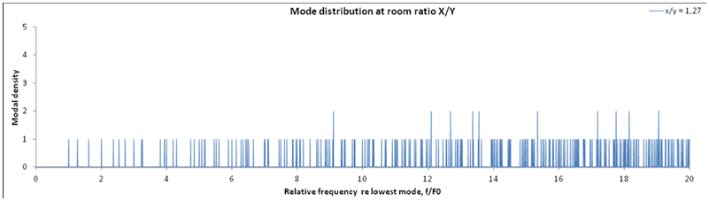
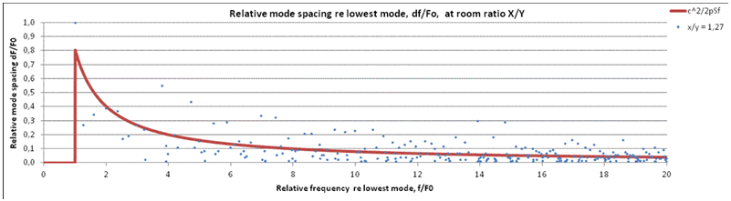
1. An example of a ratio (x/y =1.27) that creates a flat and dense modal distribution, with very few high peaks, i.e. multiple modes coinciding at the very same frequency. |
|
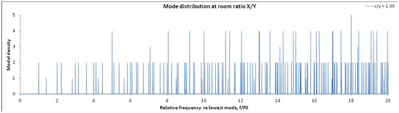
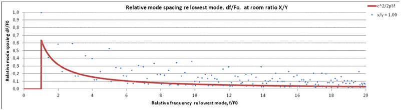
2. The square room case (x/y =1.0). An example of a ratio that creates a less flat and dense modal distribution than the ratio 1.27 in (1), with many multiple modes. |
|
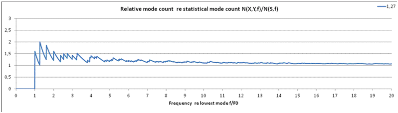
3. Actual mode count N(x/y,f) below frequency f is a function of room ratio x/y. Statistically, the mode count can be estimated from mode space considerations by the formula N(S,f)= p·S·(f /c)2 , where S=x·y is the cross-sectional area of the room. In the diagram above the actual mode count is normalized relative to the statistical mode count, the vertical axis being the dimensionless N(x/y,f)/N(S,f). The horizontal axis is the relative frequency f/f0, like in (2) and (3). Room ratio x/y=1.27 is corresponding to distribution diagram in (1). Note that actual mode count is considerably (>20%) greater than the theoretical, statistical mode count whenever relative frequency is less than 6. |
|
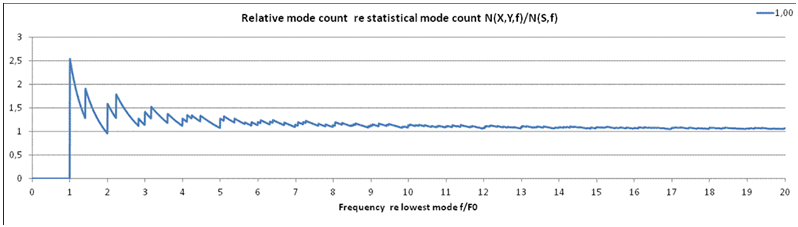
4. Same diagram as in (3), but room ratio x/y=1.0, corresponding to distribution diagram in (2). Apart from the greater fluctuations below f/f0<2, the mode count curve of ratio 1.0 is quite similar to the one of ratio 1.27 in diagram (3). |
|
5. Mode spacing plotted against frequency, with room ratio 1.27, corresponding to diagrams (1) and (3). Both axes in the diagrams have relative, unitless variables related to the lowest modal frequency of the room, f0 = 170/x. Continuous red curve represents the theoretical, statistical mode spacing deduced by derivation of the mode count N(S,f) in (3) with respect to frequency, yielding df (S,f) = c2/pSf, having taken dN=1. Zeros associated with multiple modes, which can be seen in (1) and (2) are omitted from the plot. |
|
6. Mode spacing presented as in (5), but with room ratio 1.0. Differences from ratio 1.27 in (5) can be seen, like the general tendency of larger mode spacing, and fewer dots below the statistical curve. Since the ratio 1.0 produces more multiple modes, there are more cases of mode spacing equal to zero, not being plotted. Plots in (4) and (5) shows that actual mode spacing deviates substantially from the theoretical statistical value. Toward the right of the diagram, the plot is very hard to read, since most points tends to be between 0.0 and 0.1. For this reason it seems useful to normalize the mode spacing relative to the theoretical statistical mode spacing. In the next two diagrams, relative mode spacing will instead of df/f0 be represented by df/df(S,f) |
|
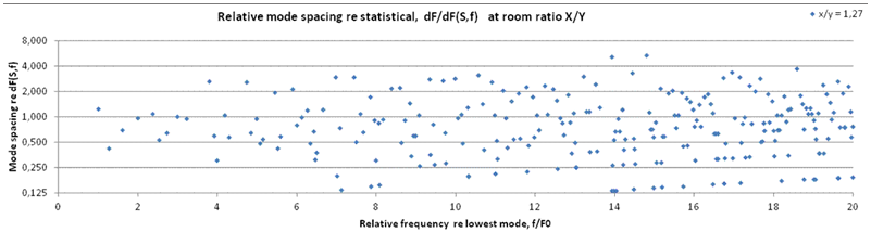
7. Relative mode spacing plotted against relative frequency, with room ratio 1.27, corresponding to diagrams (1), (3) and (5). Mode spacing normalized to theoretical statistical mode spacing df(S,f) = c2/pSf, for reasons explained above. Vertical divisions are in octaves for convenience. Deviation from theoretical value (unity on vertical axis) is exhibits random-like scattering, calling for statistical analysis. Actual mode spacing appear to be scattered within +/- 2 octaves from what can be predicted by theory, which is quite a large uncertainty in terms of room acoustics, as well as music and speech. The formations of plotted lines, slightly curved, to the bottom right in the diagram, is due to quantization effects as a consequence of computing with finite frequency resolution Df (here 0.0076), and the fact that the smallest mode spacing will be rounded off to zero or to Df . |
|
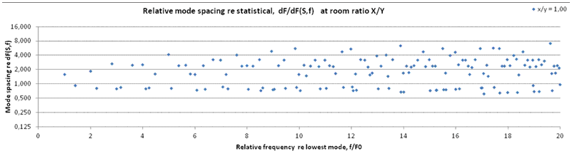
8. Like in (7) but room ratio is 1.0, corresponding to (2), (4) and (6). Compared to ratio 1.27 in (7), fewer cases of mode spacing close to the theoretical statistical value df(S,f) = 1 are seen with this room ratio. |
|
Related AKUTEK papers: Schroeder Frequency Revisited External source: Room dimensions for small listening rooms
|
|
|
|
To be continued First published 19.01.2012, latest change 27.01.2012 Go to www.akutek.info main page Go to article site index page |