Stochastic nature of room acoustics 2

The Schroeder frequency:

 f_c  ~2000·(T/V)^0.5

This is an akuTEK article by M Skålevik           www.akutek.info main page   article site index page

(1)

www.akutek.info

Background: In Stochastic nature of room acoustics Part 1 the cross-over region between the stochastic high frequency region and the low frequency non stochastic region is discussed, presenting several critical frequency candidates. In this second part, we shall concentrate on the high frequency region (2) above the Schroeder Frequency f_c (1), explore some of the important features previously pointed at by M Schroeder, and try to verify some of his results, for example:

1. The Gaussian level distribution, verified for rooms of different volume, shape and reverberation time T

2. Statistical parameters of the frequency response (FR) depend at most on T

3. Verify the approximation <D f_max > ~4/T

M Schroeder demonstrated how the importance of resolution when measuring the fine structure of the frequency response FR. Since then, the measurement apparatus and techniques have changed, and we shall study how  FR resolution depend on the length of the impulse response and the FFT time window.

Intoduction

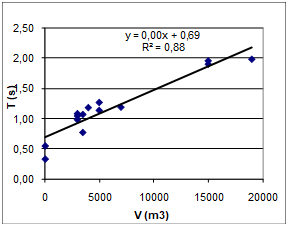
Fig 3: Reverberation time T plotted against volume V for 14 acoustic conditions, 8 rooms.

f (Hz)

dB

f_c

?

Stochastic

(2)

0.5·f_c

First published 16.05.2009, latest change 20.09.2013

Related:

Tonal response in rooms (Microstructure of room acoustic FR), a presentation by M Skålevik
Schroeder Frequency Revisited  FA 2011 presentation  29.06.2011
Schroeder Frequency Revisited  (Forum Acusticum 2011 paper) 17.04.2011

Go to www.akutek.info main page     Go to article site index page

(3)

In 8 different rooms, some of them with variable acoustics (amount of absorption), we have measured a total of 14 impulse responses (IR). From these IR’s we have  obtained 14 frequency responses (FR) through 1000ms FFT windows, implying a resolution of 1Hz. Reverberation times range from 0.3s to 2.0s, while volume ranges from 50m³ to 19.000m³, see plot in fig (3), and table (4).

A study of 8 rooms

(7)

(9)

(8)

(5)

Table 4: Room properties assosiated with the 14 frequency responses

Level distribution

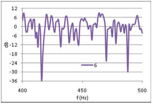
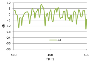
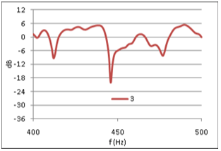
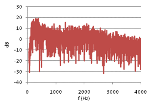
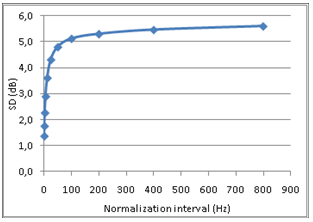
Figure (5) shows FR #6 from the opera hall, with 0dB equal to the average FR level in the range of 50-4000Hz. A combination of source power and room absorption properties, results in a general ~15dB decrease in FR level from 100Hz to 4kHz, and a sharp roll-off below 100Hz. To eliminate these non-stochastic features from the level distribution analysis, the FR is normalized as follows: For any 100 Hz wide frequency band of the FR, let the average level be 0dB, fig (6). The normalized FR’ at frequency f is equal to FR at frequency f minus the average value in the 100Hz interval where f is the center frequency. Physically this means that any effect from energy input and energy dissipation is removed from the FR. Thus FR’ describes the process of a reverberant system in energy balance.

From comparing fig (6) with fig (5) it can be seen that the normalization of FR#6 reduces the total level span just a few dB. However, the impact on the standard deviation is more significant, as the process reduces SD from 7.2dB to 5.6dB (22% reduction) in the frequency range from 50Hz to 4kHz. Eliminating non-stochastic effects is important in this analysis, thus the normalization interval should not be too wide. On the other hand, if the interval is too small it could suppress stochastic peaks with larger spacing between maxima, and alter the statistical properties of the FR. Testing the sensitivity of the FR level distribution to changing interval widths up to 800Hz revealed that standard deviation decreases strongly when normalization intervals approach zero, but is relatively insensitive to changes in intervals wider than 100Hz, Figure 13, below. A previously suggested normalization interval of 25Hz was thus rejected in favor of a 100Hz interval.

A first glance at the FR’ in 400-500Hz of three different rooms,  with reverberation times 0.37s, 1.4s and 2.1s respectively (figures 7, 8 and 9),  may indicate that the long reverberation time in (6) is associated with high peaks and deep dips. To pursue this further, we shall study the level distribution corresponding to the FR of these 3 rooms. Later, we will return to the observation that these examples seem to confirm Schroeder's theory about frequency spacing between maxima being proportional to 1/T.

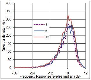
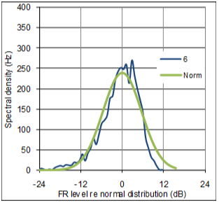
Figure (10) presents plots of spectral density vs level for FR#3, FR#6 and FR#13. Even though the three rooms are very different in volume (50 to 15.000m³) and RT (0.3s to 2.1s), their level distributions in terms of spectral density are quite similar to each other. 0dB is defined by the median level in each of the three FRs, and in the case of FR#3 and FR#13, they both have spectral density equal to 300Hz at their median levels, meaning that they have median level in 300 of the total 3950 1Hz wide bands between 50Hz and 4000Hz.

A common feature of the three distribution curves is the so called bell-shape, typical for Gaussian distribution. The asymmetry, called skewness, the steeper slope to the right of the peak, is typical for FR’s expressed in dB—and natural, since the dB scale is less sensitive to peaks than dips (remembering zero power corresponds to minus infinity in dB). 

The 50m³ listening room with low reverberation time exhibits a slightly narrower bell-shape, meaning that it’s FR has less level variation than the other FR’s. Whether this narrowness is coincidental or can be generally explained by RT will be commented below.

Figure (11) shows a comparison between the level distribution curve of FR#6 and it’s best fit normal distribution curve (Standard deviation equal to 5.2dB and median at 0dB). A prominent feature is that the curves are very similar below 0dB, while FR#6 have more median levels and less high levels than the normal distribution.

(6)

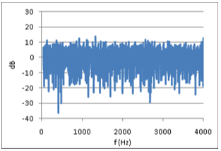
Fig 6: FR#6 normalized to 0dB in every 100Hz band

Fig 5: FR#6, 15000m³ opera hall

Comparing level distribution in FR’s of three different rooms

Fig 7,8,9: Extracts from FR’ #3, #13 and #6

Fig 10: Shape of distribution curves from three FR’s

Fig 11: FR’#6 distribution compared to normal distribution

Key properties of the level distributions of FRs 3, 6 and 13, are presented in Table 12. Explanation of FR #6: It’s standard deviation is 5.6dB; 74% of the FR levels are within the standard deviation; 45% of the levels are within +/- 3dB around the median level; at most 94% of levels are within a 20dB interval (not centered at median); and the error 3.9% is the root of the mean of the squares (RMS) of the differences between the FR distribution curve and the normal distribution curve in Figure 11.  The following features are worth noting:

· Level distribution is very close (3.9-4.8%) to normal distribution, confirming the Gaussian properties reported by Schroeder

· Sensitivity to differences in reverberation times is unclear in this limited selection, and this must be analyzed on basis of a larger number of FR’s

· Note the similarity of the distribution curves for the listening room #3 and the opera hall #6 in Figure 10, despite the great differences in volume (50 and 15000m³) and reverberation time (0.5 and 1.9s).

· Merely 45-48% of levels are within +/-3dB variation, indicating poor sound transmission quality in terms of common engineering standards, even for the quite dry listening room #3 (T~0.5s)

Correlation analysis of 14 frequency responses

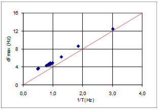
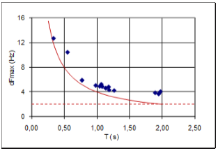
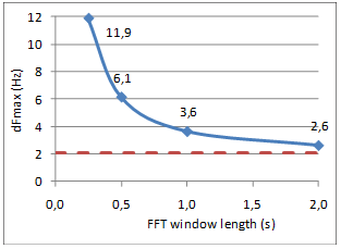
A correlation analysis has been carried out in order to reveal possible correlation between distribution parameters like standard deviation, dFmax, reverberation time T, and  the inverse of the reverberation time 1/T. Since reverberation time is calculated in octave bands , that contains more FR information in higher octaves, a weighed single number value is calculated, and denoted Tw and the inverse—(1/T)w. For example: In the calculation of Tw, the reverberation time in the 500Hz octave band is given twice the weight of the reverberation time in the 250Hz octave band. Similar weighted single numbers values are defined for other parameters in order to make them comparable with Tw and (1/T)w.

Peak spacing related to 1/T

Figure 14 is a plot of average dFmax against 1/T, both weighted, together with the line (red) corresponding to Schroeder’s  <D f_max > =4/T. The linear trend is quite prominent. All plotted values are slightly higher than 4/T, and more so towards the left of the diagram. However,  it is to be expected that dFmax can not vanish as 1/T approaches zero. Given the finite FR resolution Df=1/t, t=1.0s being the length of the FFT window, there must be at least 2Hz between adjacent maxima, thus <D f_max > can never be as low as 2Hz. In contrast to this analysis, Schroeder studied level curves from continuous signals, corresponding to higher FR resolution with Df vanishing after a long signal duration t. The lower practical limit to dFmax is demonstrated by the dashed line  at 2Hz in Figure 15, with the red hyperbola indicating the theoretical 4/T.

Figure 16 (not to be confused with Figure 15 having a different horizontal dimension) shows how the average peak spacing depends on the FFT window length. In this case we study four FRs resulting from using four different window lengths on one and the same IR, where RT=1.9s. As the FFT window length increases, the average peak spacing approaches the red dashed curve at 2.1s that corresponds to the theoretical value predicted by 4/T. When the FFT window is 2.0 seconds, approximately equal to the reverberation time, peak spacing is only 26% wider than 4/T.

We conclude that Schroeder’s <D f_max > =4/T predictor could be consistent with the average peak spacing of these measured FRs, and in particular that the general dependency of reverberation time is confirmed. Figure 16 shows that measured <D f_max >  actually approaches the theoretical value as the FR resolution  Df=1/t gets sharper, i.e. the length t of the FFT window increases. As the window length approaches infinity, FR level spectrum approaches the level spectrum of a continuous signal.

Fig 14: average peak spacing plotted against 1/T for 14 FR’s

Fig 13: SD average of 41 FRs

Fig 15: average peak spacing plotted against T for 14 FR’s

Fig 16: Sensitivity to FFT window length. RT=1.9s.

Level distribution dependency on reverberation time T

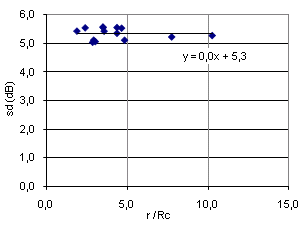
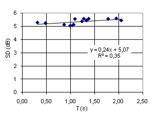
Standard deviation (SD)  is a statistical parameter commonly used as a single-number characterization of  Gaussian distribution. Figure 17 is a plot of SD values against reverberation time T for all 14 FR’s in this study (FFT window is 1.0s). As above, the FR’s are normalized to 0dB average in any 100Hz interval, the significance of the normalization interval being demonstrated in Figure 14. The linear trend of SD=0.24*T+5,07 suggests a weak increase in SD as reverberation time gets longer, and that SD approaches 5.1dB as T approaches zero. However, correlation is rather low (Pearson R²=0.35), indicating that the variation in T only partly explains the variation in SD. Low correlation is illustrated in Figure 17 by the dB-span of the trend-line being small compared to the dB-span of the measured values.  The scattering near T=1.0 calls for other explanations, e.g. measurement uncertainties. From the diagram we see that the trend predicts on average less than 0.5dB increase in SD as T increases from 0.3 to 2.3s, a range that includes the majority of rooms where acoustics is significant. Putting aside the assumption of a linear trend allows the attention to turn to the apparent transition around 1.1s, below which values are all close to 5.1dB while values are close to 5.5dB in the region of T>1.1s. This leads to the suggestion that there may be better explanations to the SD variation than the reverberation time:

Figure 18 is a plot of the same SD values as in Figure 17, but the horizontal axis is the ratio of the distance from the source (dodecahedron) to the diffuse field distance r / Rc. Along this dimension the SD values seems to exhibit a natural variation centered around the value of SD=5.3dB. Whether or not there is less degree of scatter in the rightmost region must be confirmed by collecting more data having r/Rc >5. Surprisingly maybe, the two cases belonging to the latter region are measured in the smallest room in this study. In the big concert hall r/Rc = 5 to 10 corresponds to distances 40 to 80 meter from the source, a range of distances that in practice are hardly found in this room. The “trendline” here is the best fit horizontal line. Theoretically SD=5.57 (Schroeder 1954). For SD related to r/Rc, refer to results by Jetzt (1979), see Fig 4 in this external paper by Allen and Berkley.

Conclusion: Standard deviation SD of levels from 14 measured frequency responses, with reverberation time T ranging from 0.3 to 2.0 seconds, is in the range of 5.1 to 5.6dB, with the higher values corresponding to the longer reverberation times (T>1.1s). Standard deviation appears to be best described as a statistical parameter with values scattered around some center-value that is influenced by the length of the impulse response and the FFT window, and perhaps slightly influenced by reverberation time T and the relative distance r / Rc.

Fig 17: SD from 14 FR’s, plotted against T.

Standard Deviation related to T

Percentage within +/-3dB, related to T

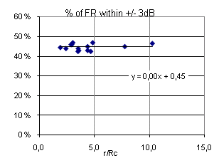
A common criteria for the frequency response of sound transmission for music and speech is that the level variation should be within +/-3dB throughout (in 100% of) the frequency range. While this criteria may or may not be an adequate criteria for room acoustical sound transmission, it can serve as a useful reference for the level variation of the FR’s in this study. Figure 19 shows the results for the 14 FR’s plotted against relative distance r / Rc. The same pattern as in Figure 18 is seen, with slightly scattered percentages (+/-2%) centered around the horizontal line corresponding to 45%, the “trendline” still being the best fit horizontal line.  In the range of reverberation times from 0.3 to 2.0 seconds, there is a weak tendency towards smaller percentage with higher T (R² =0.43).

Conclusion: For 14 measured frequency responses, 43 to 47% of the levels are within the +/-3dB interval centered at 0dB.

Fig 19: % of FR’ within +/-3 dB, plotted against r/Rc.

Percentage within 20dB, related to T

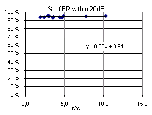
As can be seen from Figure 6, above, a 20dB range of levels is not centered at 0dB, but rather around –3 to –2dB. In the range of reverberation times from 0.3 to 2.0 seconds, there is a very weak tendency towards smaller percentage with higher T (-1% per 1 second, and R² =0.39). An analysis (Figure 20) similar to the one of the +/-3dB interval above leads to the following conclusion:

For 14 measured frequency responses, 93 to 95% of the levels are inside a 20dB interval centered at –2 to –3dB.

Fig 18: SD from 14 FR’s, plotted against relative distance  r/Rc.

Fig 20: % of FR’ within 20 dB, plotted against r/Rc.

Share this:

HOME

INDEX