Go to www.akutek.info main page     Go to article site index page

Introduction to Ensemble Acoustics

Background

This page is motivated for in  the article Music Room Acoustics.

Room acoustical ensemble play response should not be confused with room acoustical solo play response

Ensemble acoustics and acoustics for solo play is not generally the same. Acousticians judging every hall by singing, shouting, clapping their hands, or assessing impulse response measurements, should keep in mind that they actually judge the acoustic conditions for a solo musical performer. To judge ensemble performer conditions, impulse responses must be analysed with experience or by methods taking the difference between soloist acoustics and ensemble acoustics into account. A point source is seldom a useful model for the ensemble source. Neither does the early-late time integration limits have the same meaning. E.g., evne if all musicians play perfectly in sync with the conductor, the direct sound from an instrument 10m away from the conductor and a 30ms delayed reflected sound from an insturment nearby would arrive simultaneously at the conductor.

The introduction below focuses on listening conditions on stage, but an extension to listening conditions in the auditorium could be relevant.

Ensemble Acoustics

Sound from an ensemble, i.e. a music group of any size N>1 in general and an orchestra in particular, can be analyzed in different ways. One way is to analyze from the individual musician’s perspective, see matrix above, into Dry Self (an-echoic sound of own instrument), Dry Others (an-echoic sound of other instruments) and Dry All (reverberant sound of own and other instruments). These three components can be combined into the categories Foreground-Background and Dry-Reverberant. This approach is pursued under the section Parallel streams below, after a more detailed discussion of the elements of ensemble sound. Readers who would like to save details for later can jump to Parallel streams.

1. An-echoic sound  from the individual instrument

2. Early ensemble sound (sum of all sound arriving no later than 80ms after first sound arrival)

2a. Early an-echoic sound from the ensemble

2r. Early reflected sound from the ensemble

3. Late ensemble sound (sum of all sound arriving later than 80ms after first sound arrival)

3a. Late an-echoic sound from the ensemble, i.e. reverberant sound in the instruments

3r. Late reflected sound from the ensemble

Part 1 is the sound one would hear from the individual instrument if the ensemble was placed on a hard floor in an-echoic environment. This part is the part of sound that makes the performer able to hear one’s own instrument, and co-players and listeners able to localize and identify individual instruments. In usual simplification, Part 1 is taken equal to the direct sound in free field radiation. However, in general this is not correct, since we must consider obstruction, diffraction, absorption and reflections from persons, instruments, music stand and floor, i.e. all acoustical elements present in any environment where ensemble music is performed. 

Part 2 is the blend of two early sound parts, 2a and 2r. Part 2a is the early sound one would hear from the ensemble if it was placed on a hard floor in an-echoic environment. It is the sum of the N individual parts included in Part 1. Part 2r is the sum of early reflected sound from the N instruments of the ensemble. In practice, it will be difficult to separate Part 2a or Part 2r from the total of Part 2, except for the sound from the nearest instruments. The significance of Part 2r is that it determines the perceived loudness of early sound, since Part 2a is naturally weak. 

At performer’s position, the level balance between Part 1 and Part 2 is important in order to be able to discriminate one’s own instrument from the ensemble instruments. At listener’s position there will be a negative level balance between Part 1 and Part 2 in the typical ensemble play case. However, in solo play, it is important that this level balance is not too low.

Part 3 is the blend of the two late sound parts 3a and 3r. Typically, late ensemble sound is dominated by 3r, which is the sum of late reflected sound from the N instruments of the ensemble. However, in general one must keep in mind that Part 3 is a blend of late reflected sound in the room (3r) and the sum of reverberant sound (3a) in the N instruments. Given the common early to late sound time limit, any residual vibration more than 80-100ms after the end of a musical note will add to part 3a. This time is just 1/10 of a second and corresponds to the duration of a 1/16 note or pause in tempo 150 bps, which is really fast playing. In practice, there is no abrupt end to a note played on a physical instrument, and in fact, the musician-controlled decay of the sounding instrument is an important part of musical articulation, e.g. legato, portato, staccato and so on. 3a creates temporal continuity in the ‘voice’ of the instrument by tying together subsequent notes, and 3r is the room acoustical addition to this continuity.

An important significance of Part 3 is to provide a sounding background for the music being played. Late sound from the previous note sounding together with the present note creates harmonic effects similar to those associated with chords, dissonances, consonances, and transition effects like harmonic tension and relaxation. If too much Part 3, the whole sound will be muddy. For example, while arpeggio-like passages of thirds or greater intervals sound clearly like chords, a diatonic scale-like passage may, if Part 3 is too strong, become constantly dissonant due to the presence of more than one spectral component inside each critical band. In live rooms where Part 3r is relatively strong, musicians will tend to reduce Part 3 by applying a more staccato-like style of play, which has a double effect on Part 3: More abrupt note endings provides less energy to Part 3a, and shorter note duration provides less energy to Part 3r (reverberant buildup level depends source duration for duration shorter than T/20, the time to build up to 3dB below maximum, T being the classical reverberation time). This technique is important for organ and singers in choral music, due to long T common in the cathedrals where such music evolved.

While Part 3a basically is determined by the composer, and modified by interpretation under the control of conductor and musicians, Part 3r is determined by the room alone. In general musical styles have evolved together with the environment provided by spaces large enough to house orchestra and audience of certain proportions.

To some degree it is possible for trained musicians to compensate with more legato-like play for the lack of late reverberant sound in too dry performance spaces, thus increasing the contribution to late ensemble sound from Part 3a. However, this effect will not provide the sound quality of a late ensemble sound dominated by late reflected sound, and for the musician and conductor aiming to express the music according to ideals or composers intention, such compensation means lack of freedom, not to mention the effort it takes.

Part 3r is assumed to dominate the perception of Envelopment (ENV). In the auditorium, Part 3a can be discriminated from 3r by localization, and contribution to ENV from Part 3a is uncertain. On stage, especially inside the ensemble, Part 3a is assumed to contribute to performers envelopment.

Except for Part 3r, which varies moderately throughout one and the same room, all parts 1 thru 3a vary greatly from performer’s position to listener’s positions. For this reason, Part 3r is the only part able to feed back information about the ensemble sound quality reaching out to listeners’ ears.

Compared to the other parts, Part 3r of sufficient amount provides a more invariant reference for intonation, since intonation and pitch detection becomes more certain with longer tone duration. For the musician, Part 3r extends the duration of the tonal reference. 

It has been suggested that Part 2 and Part 3 can be perceived as two separate streams of information, associated with source presence and room presence, respectively.

Parallel streams
Parallel streams of information could be divided in two alternative ways that are considered relevant to the ensemble musician, namely Foreground versus Background, and Dry sound versus Reverb sound, see matrix above.

Foreground-Background
It is assumed that in the ensemble musicians total sound image, the dry component of one’s own instrument is in the Foreground stream, while other instruments and reverberant sound are in the Background stream. In some cases it would be relevant to subdivide the background, considering other instruments in one’s own voice group (playing in unison) as Middle Ground, while the remaining instruments are considered Background. Based on the analysis above, a simple division into Foreground stream and Background stream, the level balance between the two streams could be expressed as follows.

Foreground-Background-Balance FBB = 10*log[SPL(A)] - 10*log[SPLsum(B,C)]

Dry sound versus Reverb sound
Some results from simulations [1] and measurements [2]  have shown that the balance between the anechoic (Dry) sound stream and the reverberant (Reverb) sound stream  can be consistent throughout very different spaces for different purposes in the range from individual rehearsal to orchestra performance.  In contrast, the Dry-Reverb-Balance DRB would tend to deviate whenever the room acoustics was not adequate for the actual use. Hence, the potential of DRB as a possible “indicator of proper acoustics” is to be investigated in further work.

Dry-Reverb-Balance DRB = 10*log[SPLsum(A,B)] - 10*log[SPL(C)]

In the simplest case, an unobstructed point source, the DRB would be equal to the commonly used Direct-to-Reverberant level D-R.

Dry sound from ensemble (B or 2a+3a)

Considering the ensemble of N musicians and instruments contained by an imaginary box, a prism to be precise, having height H at typical ear height for seated musicians. The prism base is formed by a floor of area S , its volume is H∙S and its perimeter can be estimated by P=4.1∙S^0.5. Longest diameter within the prism is estimated by 1.6∙S^0.5 . Letting all N sources start simultaneously at t=0, it is assumed that after the propagation time t_d=1.6∙S^0.5/c of the longest diameter, the sound field on the box surface has built up to steady state. If the average floor area per musician is S/N the prism surface area through which the ensemble power is emitted equals S’= S + H∙4.1∙S^0.5.

Example 1: If the ensemble density is given by the common S/N = 1.5m² per musician, and the ensemble is smaller than N=100, the estimated propagation time along the longest diameter will be less than t_d= 58ms. With H=1.2m the ensemble emission surface equals S’= S + 4.9∙S^0.5 , having the critical base area S~24m2, and ensemble size N=16, below which the perimeter surface dominates the emission.

Now the total emitted power from the ensemble is N∙w, where w is the average power emitted per musician. Due to symmetry the steady state intensity vector is assumed to be normal to the surface S’ and its size I₀ = N∙w/S’. Thus the power w emitted per musician may be weaker than the power w₀ emitted from the average instrument, since musicians with their chairs etc absorb sound. Given the solid angle W of the ensemble, as seen by the average instrument, we denote the fraction of source power emitted in to the ensemble by g = W/4p. Given the random incidence absorption factor of the ensemble, a, the fraction of source power lost in the ensemble is ag, while the fraction of source power emitted from the ensemble box is 1- ag. Thus the emitted power per musician is w = w₀(1- ag) and the intensity normal to the box surface equals

I₀ = N∙w₀(1- ag)/S’ 

Example 2: Assuming that a large ensemble, seen by the average instrument, covers 70% of whole-space, g = 0.7, and the absorption factor for an ensemble at mid-frequencies equals a=0.8 (ref: ODEON material database), the emitted ensemble power per average musician becomes w = 0.56∙w₀ . In the case of N=80, H=1.2m, and S/N=1.5m² , S equals 120m² , and the ensemble surface intensity becomes I₀ = 80∙w₀(1-0.56)/(120+4.9∙120^0.5) = 0.203w₀ (W/m²).  In the case of a quartet, N=4, the solid angle of the ensemble, seen by the average instrument, is quite small, assuming  g = 1/8, thus the ensemble surface intensity becomes I₀ = 4∙w₀(1-0.8∙1/8)/(6+4.9∙6^0.5) = 0.200w₀ (W/m²).

Note that the emitted ensemble power is approximately 3dB less than the total power of from the instruments, due to absorption  (w = 0.56∙w₀ ).

Comment to Example 2: Given the approximately equal results of ensemble surface intensity, I₀ =0.2w₀ (W/m²), in two extreme examples of ensemble size, N=80 and N=4, despite very different perimeter surface to base surface ratios, may indicate that increased g  of a large ensemble is balanced by reduced “perimeter leak”, and vice versa. The resulting intensity is equal to free-field intensity at distance 0.63m from the average instrument, which is then the average critical distance for intensity balance between own instrument intensity and ensemble intensity.

Reference level: As usual we want to describe sound levels at various locations relative to some reference level.  Above, we deduced the ensemble surface intensity relative to the average power from the average instrument, w₀ . However, the instrument power would be an impractical reference if it turns out that the effective power emission is reduced by the presence of the musician or the ensemble.  Thus we need to define the average musician with the average instrument together as the sound source. We see at least two possible reference source candidates, namely 1) the average soloist in an unobstructed, freely radiating position on stage, and 2) the average musician located in an ensemble.  Which one to choose? Both ones appear to be relevant.

Reference source candidate 1) is a simple and basic candidate, and the one that directly provides measures of the difference between solo response and ensemble response. Since acousticians often test the solo response by clapping, shouting, singing and impulse response measurements and predictions, the soloist reference may be very useful. This power is the power emitted during individual practice, and the only measureable power.

Reference source candidate 2) seems to be justified by the fact that ensemble acoustics is the issue here.

In the following, source candidate 1), the soloist reference, is chosen due to the reasons above. It is assumed that the musician would represent an absorbing surface with a=0.8 , covering 1/8 of the solid angle as seen by the average instrument. Thus g = 1/8, and the power emitted by the average soloist is w_ref = w₀(1- ag) =  w₀(1-0.8∙1/8) = 0.9∙w₀ .

At 10m free-field distance from the reference source, the intensity is I_ref,10m=  w_ref /(4p10²)  =  0.9∙w₀ /(4p10²) . Now, given this equation, the surface intensities of Example 2 could be expressed approximately as follows: I₀ = 4p∙10²∙0.2∙w₀ /0.9∙I_ref,10m ≈ 280∙I_ref,10m . The average intensity at the surface of the ensemble is 280 times the intensity at 10m free-field distance from an individual ensemble instrument, corresponding to 24.5dB level difference. If the reference source  is represented theoretically by a point source, the surface intensity of the ensemble is equal to the intensity at 0.6m free field distance from the reference source.  At distances closer than 0.6m to the average individual instrument, assuming point source similarity, the intensity from the individual instrument would be stronger than the intensity from the ensemble.

Since instruments are not real point sources, we define the apparent distance from a real source r’ = [w/(4p∙I_d)]^0.5 , where I_d is the dry (anechoic) intensity from a real source emitting the power of w. Note that reflections from floor and music stands etc. would be included in our concept of “dry”, and could contribute to a shorter r’ than a pure free-field (4p radiation) case.

Average vs varying source power
Values from the expressions above apply to sound from the average instrument in an ensemble, and would apply directly to an ensemble with equal instruments playing in unison. For real orchestras, the values have to be corrected for the variation in power of the actual instruments in scope. E.g., since the violin is weaker than the average source, one must expect that the violin-to-violinist’s-ear distance must be kept shorter than average in order for the violinist to achieve the same Foreground-Background balance, FBB, as the average ensemble musician. Indeed, this seems to be the case in common violin play. On the other hand, for more powerful instruments, this distance must be longer than average in order to achieve a proper FBB, and probably in order to avoid hearing damage, too.

In general, the power of the individual instrument could be expressed w_i =k_i∙w₀ , where k_i is a the power constant and  w₀ is the power of the average instrument.

Intensity components, diffusivity and energy density

In a plane wave where the sound pressure is p , intensity I=p²/rc, and the characteristic impedance rc , the energy density is e =I∙c

In the case of a diffuse sound field, the energy density is e =4∙I∙c

In general, if diffusivity is denoted D, the energy density is  e =D∙I∙c

The combined energy density of two sound fields would be e =e₁+e₂ =(D₁∙I₁+D₂∙I₁)∙c

Foreground-Background-Balance FBB
The foreground intensity at the ear of the musician playing the i-th instrument is I_i,F=k_i∙w₀ /4p∙r’² , where r’ is the apparent instrument-to-ear distance.

The anechoic part of the Background intensity from the ensemble is  I_B =0.2∙w₀

The reverberant part of the Background intensity is I_r = N∙w₀ /A = N∙6.25∙w₀ ∙T/V

Diffusivities are D_i,f, D_B and D_r, and  in terms of energy densities FBB= 10∙log[ e_i,F /(e_B + e_r) ]

Combining expressions above, w₀ would be cancelled, and FBB=10∙log(D_i∙k_i /4p∙r’² ) –10∙log(0.2∙D_B+6.25∙D_r∙N∙T/V)

Example:  Assuming k_i =0.5, r’=0.25,  N=80, T=2.0s, V=20.000m³, and diffusivities D_i,F =1, D_B =1.5 and D_r =4.

FBB=10∙log(0.64) –10∙log(0.3+0.2) = +1.0dB

Dry-Reverb-Balance DRB

If applying the same assumptions as in the FBB example above, N=80, T=2.0s, V=20.000m³, the Dry-Reverb-Balance would be

DRB=10∙log(D_i∙k_i /4p∙r’² +0.2∙D_B) –10∙log(6.25∙D_r∙N∙T/V)=10∙log(0.94) –10∙log(0.2) = +6.7dB

Examples with other power factors k_i and apparent instrument-ear-distances r’, producing different FBB and DRB below. In these pie-diagrams, the balance between the energy density components are highlighted. Self=Foreground, Self+Others=Dry, Others+Reverb=Background. Values are energy densities, where 1.0 would be the energy density from the average instrument at distance r’=0.28m.

Note that the total energy density at the ear of the musician is dominated by the Foreground (Self), i.e. his/her own instrument, even if N=80:

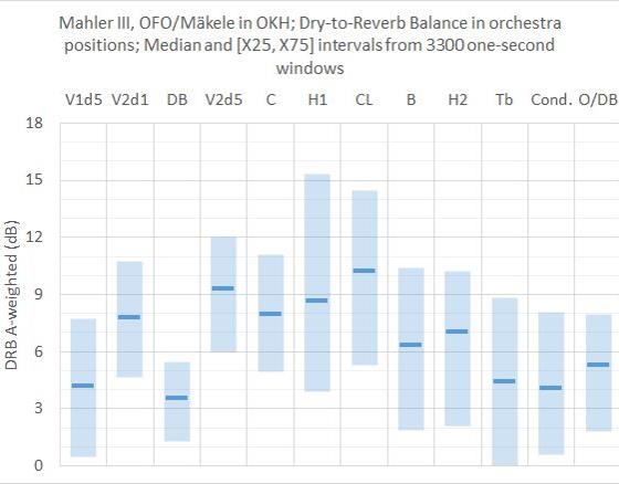
A-weighted Dry-Reverb-Balance DRB(A) in a symphony orchestra estimated from measurements

The level balance between the total sound from orchestra instruments and the sound reflecting from the room, i.e. the Total-to-Reverb Balance, was calculated from 15 measurements points during a performance of Mahler 3rd Symphony in Oslo Concert Hall (OKH) with Oslo Philharmonic Orchestra (OFO) conducted by Klaus Mäkele in May 2022.

10 of the measurement points were dosimeters mounted close to the ears of musicians, distributed over the orchestra.

One microphone (#2) was 1m above the floor close to 1st violin 1st desk, 2nd violin 1st desk and the conductor. One (#3) was 1m above the floor between oboe section and double bass (DB) section. One (#5) was 1m above the floor behind the  rear row with timpani and misc. percussion. Two microphones were placed at 20-24m distance from stage center. #7 was in Row 30.

All microphone signals were synchronized in post-processing by optimizing their cross-correlations.

Equivalent sound pressure levels LpEq were sampled in 3300 windows of 1 s duration in all signals. In post processing A-weighting and third-octave analysis was calculated.

The level of the room response on stage was estimated for each second from measurement data from #7 in Row 30, and corrected by 0.176*d/T according to Revised Theory, where d is distance from stage and T is reverberation time. From simulations in a 3D model it was made sure that #7 in Row 30 was dominated by reverberant sound even in parts with directive brass instruments.

From the Total-to-Room Balance, the Dry-Reverb-Balance DRB can be calculated.

Results from calculated Dry-Reverb-Balance, DRB, are given in the diagram below. V1d5= 1st violin 5th desk, V2d1 = 2nd violin on 1st desk, DB= double bass, V2d5 = 2nd violin on rearmost desk in front of woodwinds,  C=Cello, H1 = horn with bell of other horn to the left, CL= clarinet, B=Bassoon (contra), H2= leftmost horn in horn section (less exposed), Tb= trombone, Cond= conductor/V1/V2 (#2), O/DB= between oboe and double bass (#3).

Bars indicate the middle range between X25 and X75, i.e. between lower and upper quartiles respectively, containing a horizontal marker indicating the median, i.e. X50, the 50-percentile.

Comment: In V1d5, DB and Tb, the dry sound from the instruments is on median close to 4dB above the room response in the 3300 one-second windows. These instruments are all placed in the outer parts of the orchestra. Other instruments are more surrounded, thus more influenced by dry sound from others, showing median values ranging from 6 to 10dB.  DRB=0 dB  would mean that the level of reflected sound is equal to the dry sound from the orchestra instruments. In Tb, dry sound is weaker than reverb sound in 25% of the time during the symphony, as can be seen from the bar touching DRB=0dB. 

Simulations of a symphony orchestra in Odeon and in-ear measurements on a violin player while playing in an orchestra  https://akutek.info/Papers/MS_Consistency.pdf , together with the study of the theoretical model above, indicate that DRB values in the 6-8dB range can be expected in good rooms.  The current results from measurements on many different instruments in very different positions shows a wider range of 4-10dB, and the average instrument (N=10) has a median of DRB=7.8dB. In order to evaluate the results further, we need more data.

An analysis based on Wenmaeker’s theoretical model resulted in 34% reverberant sound, i.e. DRB=3 dB, for the average instrument, page 12 in this document https://www.akutek.info/Presentations/MS_orchestra_ASA_2019.pdf . This is lower than the other results reported above.

Another way to study the current result, is to estimate the percentage of time during the symphony that the Reverb sound component is stronger than the Dry sound component, as presented in the table below. This happens more frequently in the “corner positions” V1d5=22% and Tb=27%, and rarely in the middle of the orchestra, V2d5=6%, C=7% and CL=7%. The difference between V2d1=8% and Conductor=21%, at almost equal positions, is probably because the latter microphone is not mounted on a musician.

Instrument / Position	V1d5	V2d1	DB	V2d5	C	H1	CL	B	H2	Tb	Cond.	O/DB
Reverb stronger than Dry	22 %	8 %	16 %	6 %	7 %	9 %	7 %	17 %	18 %	27 %	21 %	17 %

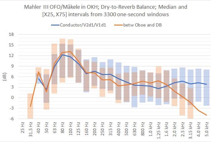
DRB in third-octave bands 25-5000Hz

Further to the results in the section above, a frequency analysis was performed.

The diagram below shows the Source-to-Room Balance for the two points #2 “Cond” and #3 “O/DB” in all third  octave bands from 25Hz to 5kHz, with Median and mid-range bars for [X25,X75].

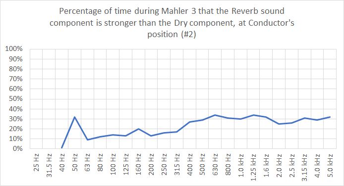
Comment: Comparing these results with the A-weighted single-number DRB(A) above, DRB(A) = 4dB for #2 (Conductor++) and 5dB for #3 (Oboe-DB), reveals interesting details in the frequency spectrum.

Dry sound is more dominating at low frequencies, peaking with some 12-13dB in 80-100Hz. With a median above 10dB in 63-125Hz, reverb sound is not audible in an important part of the bass region in these two positions.

From the mid-range bars above 315Hz, we note that in 25% of the time during the symphony, reverb sound is stronger than the dry sound from the orchestra instruments, because DRB<0dB (mid-range bars extend below 0dB).

The two microphone points exhibits quite similar and overlapping results, except for above 1.6kHz where the Conductor position is more dominated by dry sound from violins, while the Oboe/DB position is more influenced by the room response.

The diagram below shows the percentage of time during the symphony that the Reverb sound component is stronger than the Dry sound component at Conductors position. In the 400-5000Hz range, this happens around 30% of the time, while in the bass region, except at 50Hz, it happens down to 10% of the time.

Relevant links: Music Room Acoustics; Consistency in music room acoustics; Rehearsal room acoustics for the orchestra musician,

To be continued

First published 26.02.2012, latest change 06.01.2023

Go to www.akutek.info main page     Go to article site index page