|
Directivity of musical instruments |
|
Go to www.akutek.info main page Go to article site index page Introduction This page reports from AKUTEK research on directivity of musical instruments. Progress is presented and explained chronologically in numbered sequence below. Unlike loudspeakers, many musical instruments do not in general have a defined axis around which the radiated intensity is maximized at all times. And for those instruments who have a defined axis, e.g. trumpets, the axis will move as the musician moves while playing. As a result, at any receiver position, the spectrum from a hand held instrument will in practice vary with time, even if the exact same note is repeated. While the static directivity of a loudspeaker can be described by the ratio of axial intensity to the average intensity over all directions, we shall for the purpose of this investigation define the time-variant directivity of musical instruments as follows: 1) At frequency f, in any finite time window [t-t , t] time t and of length t , the time– and Directional Radiation Level DRL(f,t,t,θ) is the instant intensity level in direction θ, in dB relative to the level of average intensity over all directions. When t=t → ∞ , DRL is equal to the long-term directivity pattern. DLV(f,t,t,N) = Standard Deviation of DRL(f,t,t,θ) measured in N directions θ1 ....θN at frequency f during the time period [t-t , t] Due to the normalization of average intensity set to 0dB, the time-varying total emitted power does not influence on DRL(f,t,t,N). Thus, DRL is a measure of the directional unevenness at frequency f and time t. If t is small, DRL is a measure of the instant directional unevenness at time t. 3) At frequency f, in any direction θ, the Temporal Level Variation TLV of measured DRL’s in M periods of length t , is defined by TLV(f,t,θ,M) = Standard Deviation of DRL(f,t,t,θ) measured in M periods t1 ....tN at frequency f in direction θ
|
|
Summary The 5 channnels of the investigated D5 note can be heard in sequence in this wav-file http://akutek.info/wav/m_1st_violin1_5ch_sequence.wav
|
||||||||||||||||||||||||||||||||||||||||||||||||||||||||
|
|
||||||||||||||||||||||||||||||||||||||||||||||||||||||||
|
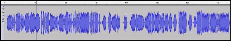
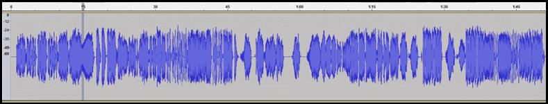
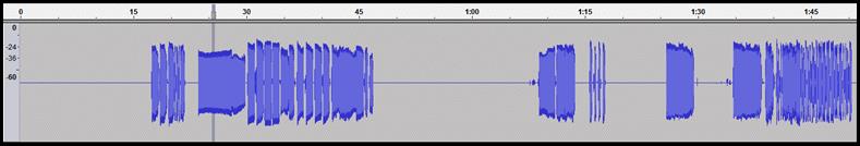
1. Wave-form (dB) versus time, anechoic recording of Violin 1 in front of player (ch1), first 1 min and 50 sec of Mozart Symphony No 40, G-minor |
||||||||||||||||||||||||||||||||||||||||||||||||||||||||
|
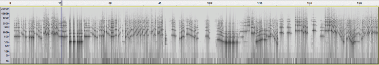
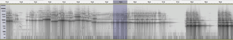
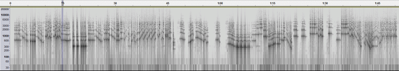
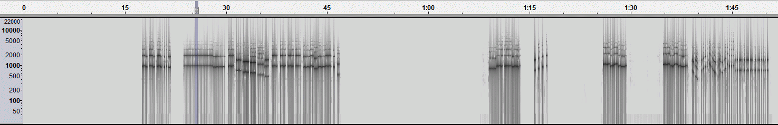
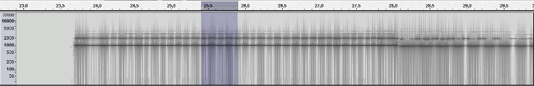
2. Spectrogram corresponding to the wave-form in Fig 1. The grey-marked 500ms period at 15s280ms is subject to more detailed analysis below |
||||||||||||||||||||||||||||||||||||||||||||||||||||||||
|
|
||||||||||||||||||||||||||||||||||||||||||||||||||||||||
|
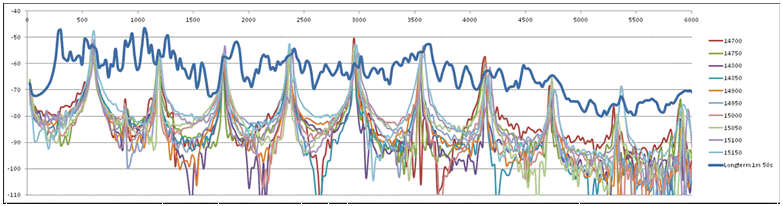
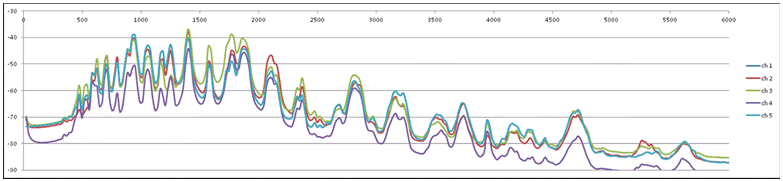
4. Spectrum of ch 1, long-term spectrum (bold curve) and ten 50ms-window spectra between 15s 280ms and 15s 780ms; FFT size 2048. The upper harmonics are smeared out in frequency due to the slight vibrato, see Fig 3. Components higher than –6dB relative to long-term level in all 5 channels are selected for the directionality analysis below. |
||||||||||||||||||||||||||||||||||||||||||||||||||||||||
|
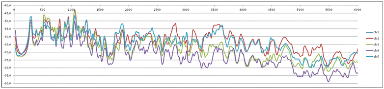
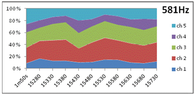
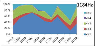
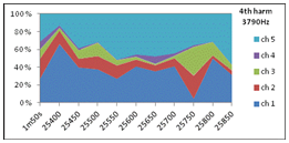
5. Dynamic directivity at 1st and 2nd harmonic of D5, area diagrams showing instant intensity per channel varying along the horizontal time-axis (in ms), through the ten 50ms windows. ”1m50s” leftmost in the diagram indicates the long-term average. 20% correspons to the average intensity of the 5 channels. At 581Hz (1st harmonic of D5) the intensity variation over time and directions (channels) are considerably less than at 1184Hz (2nd harmonic of D5). Variation statistics of this data is presented in 6a (temporal variation) and 6b (directional variation) below. Note the dramatic shift in main radiation pattern of the 2nd harmonic (1184Hz) seen if comparing ch1/ch5 levels at 15380ms and 15680ms. |
||||||||||||||||||||||||||||||||||||||||||||||||||||||||
|
6a. Statistics from Fig 5. Temporal level variation TLV in each of the five direction (channel) in terms of standard deviation of intensity levels in M=10 periods of 50ms length. A plot of the whole frequency range is presented in 7a below.
|
||||||||||||||||||||||||||||||||||||||||||||||||||||||||
|
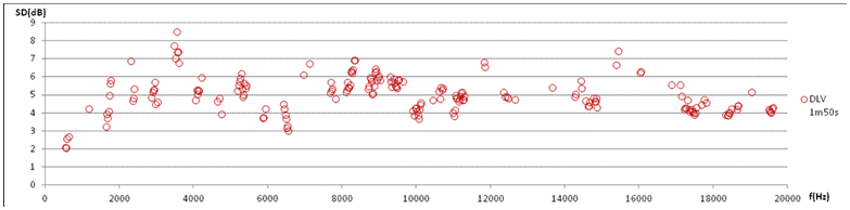
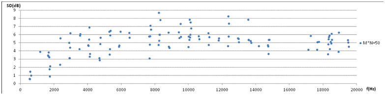
6b. Statistics from Fig 5. Directional level variation DLV in each of the ten 50ms periods, in terms of standard deviation of intensity levels in five directions (channels). Longterm DLV in leftmost column for comparison. A plot of the whole frequency range is presented in 7b below. 6a-6b comparison: Level variation over instants is comparable to variation over direction in 1st harmonic (581Hz band) as well as in the second harmonic (1184Hz band). The tendency of generally increasing variation with frequency will be investigated further. This indicates that variation over directions is of the same nature as variation over time. 6c. Level variation over the whole data of size M*N=10*5=50 exhibits a standard deviation of 0.8dB in the narrowband centered at 581 Hz, while 4.6dB at 1184Hz. Level variation of all harmonic components are plotted in 7c below. |
||||||||||||||||||||||||||||||||||||||||||||||||||||||||
|
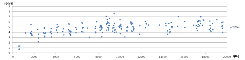
7a. Temporal level variation TLV in terms of standard deviation of M=10 periods (t=50ms), average of five directions plotted against frequency. TLV rises steeply above the fundamental. Above 5300Hz (9th harmonic) the TLV appears to fluctuate around an average of 5.2dB. |
||||||||||||||||||||||||||||||||||||||||||||||||||||||||
|
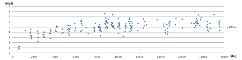
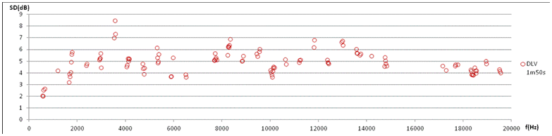
7b. Directional level variation DLV in terms of standard deviation of N=5 directions, average of 10 periods (50ms) plotted against frequency. DLV rises steeply above the fundamental. Above 5300Hz (9th harmonic) the DLV appears to fluctuate around an average of 5.5dB. |
||||||||||||||||||||||||||||||||||||||||||||||||||||||||
|
|
||||||||||||||||||||||||||||||||||||||||||||||||||||||||
|
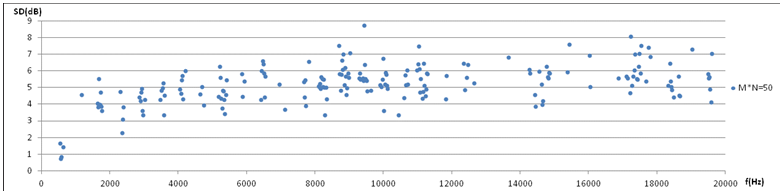
7d. Level variation in terms of standard deviation of the whole set of size M*N=10*5=50 plotted against frequency. The same trend as in 7a and 7b is seen, but above 5300Hz (9th harmonic) the level variation appears to fluctuate around an average of 5.6dB. |
||||||||||||||||||||||||||||||||||||||||||||||||||||||||
|
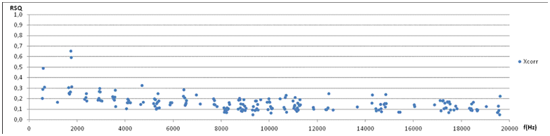
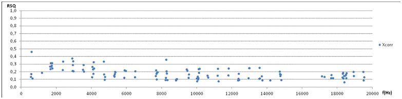
7e. Correlation (Pearsons r2) between the 5 channels, average of the10 pertubations 1-2,1-3,1-4,1-5,2-3,2-4,2-5,3-4,3-5,4-5., plotted against frequency. Average over the whole frequency range is low, r=0.16, with increasing values towards 0Hz, consistent with the observation of random-like radiation at higher frequencies, and coherence at lower frequencies. No sharp transition is seen, but the highest value below 2kHz is more than twice the highest value above 2kHz. |
||||||||||||||||||||||||||||||||||||||||||||||||||||||||
|
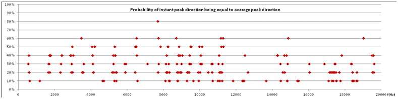
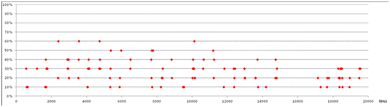
8. Peak radiation. The peak direction is the direction in which the radiated intensity is the strongest. The plot displays probability of the instant peak direction being equal to long-term average peak direction. On a probability scale from 0 to 100%, 100% would mean that peak radiation was constantly equal to long-term average peak direction, and 20% would indicate that peak direction is perfectly random. Average probability over the whole frequency range is 26%, meaning that peak direction is relatively close to random over the 10 analyzed instants. In this context, an ”instant” is a time window of 50ms. |
||||||||||||||||||||||||||||||||||||||||||||||||||||||||
|
9a. Comment: Even if the set of TLV above 5300Hz is statistically significant (p=0.04) from the set of DLV in the same frequency range, TLV and DLV is highly correlated, r=0.93. DLV and TLV correlates higher with the whole data set, r=0.95 and r=0.94 respectively. TLV is not significantly different from whole data set (M*N). 9b. Tentative conclusion: Both the temporal and directional level variations are random outcomes of a stochastic prosess at higher frequency, however tending towards zero variation as frequency approaches 0Hz. Level variation values at higher frequencies (SD=5.2-5.6 at f>5300) is very close to those found in room acoustic frequency response (http://akutek.info/articles_files/stochastics_2.htm), leading to the question: Do the overlapping reverberant modes of a violin body create the same kind of level fluctuations as those created by overlapping room acoustic modes, like in a Gaussian process described by Schroeder? If it had not been for the clear tendency towards SD=0dB as f->0, one could suspect the whole data set to be just random outcomes of the measurement and analysis process. However the small variance at the lowest harmonics clearly tells a different story: At low frequencies the fluctuations vanish, which can be explained by increasing phase coherence and fewer, or no, overlapping modes. Towards 0Hz kD would approach zero for any internal distances D on the violin body, k being the wave number of structural bending waves, eliminating any possible multipole or even dipole radiation. 9c. Further work: One might suspect that the random-like level variation observed and reported above, and the deviation from long-term directivity in particular, could be a special case for some reason. As a hypothesis, the prominent vibrato seen in (3) is suggested to be a possible cause of rapid changes in radiation pattern. Therefore, a similar data set (data size M*N=10*5, same 50ms windows, same number of channels and periods, with the sam note D5, only played without vibrato, will be analyzed in the same manner as above. Steps 1-10 will be repeated with the different data set and reported in sequence, in numbered steps 11-20 below. Note that the D5 note analyzed below is intonated slightly higher than the D5 note analyzed above, fundamental peaking at 603Hz rather than 581Hz.. |
||||||||||||||||||||||||||||||||||||||||||||||||||||||||
|
11. Wave-form (dB) versus time, anechoic recording of Violin 1 in front of player (ch1), first 1 min and 50 sec of Mozart Symphony No 40, G-minor |
||||||||||||||||||||||||||||||||||||||||||||||||||||||||
|
12. Spectrogram corresponding to the wave-form in Fig 11. The grey-marked 500ms period at 14s700ms is subject to more detailed analysis below |
||||||||||||||||||||||||||||||||||||||||||||||||||||||||
|
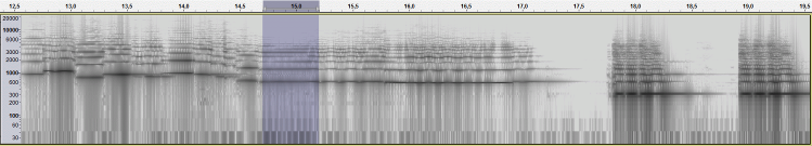
13. Spectrogram of the period 12.5s to 19.5s, zooming in on the analysis period during a single D5 note (592Hz) without vibrato |
||||||||||||||||||||||||||||||||||||||||||||||||||||||||
|
14. Spectrum of ch 1, long-term spectrum (bold curve) and ten 50ms-window spectra between 14s 700ms and 15s 200ms; FFT size 2048. All harmonics are more narrow-banded and collected than those in (4), due to vibrato-free intonation, see Fig 13. Components higher than –15 dB relative to the long-term spectrum in 5 channels are selected for the directionality analysis below. |
||||||||||||||||||||||||||||||||||||||||||||||||||||||||
|
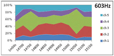
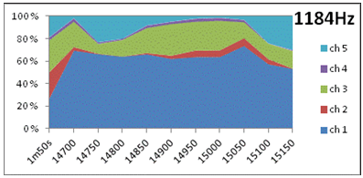
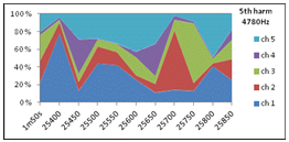
15. Dynamic directivity at 1st and 2nd harmonic of D5, as explained in (5). At the1st harmonic of D5 (603Hz), the intensity variations over time and directions (channels) are slightly greater than in (5), while slightly less at the 2nd harmonic of D5 (1184Hz) . Both harmonics deviate considerably from long-term radiation throughout the analysis period. Variation statistics of this data is presented in 16a (temporal variation) and 16b (directional variation) below. Note the dramatic shift in main radiation pattern at 15050 ms. |
||||||||||||||||||||||||||||||||||||||||||||||||||||||||
|
16a. Statistics from Fig 15. Temporal level variation TLV in each of the five direction (channel) in terms of standard deviation of intensity levels in M=10 periods of 50ms length. A plot of the whole frequency range is presented in 17a below. |
||||||||||||||||||||||||||||||||||||||||||||||||||||||||
|
16b. Statistics from Fig 15. Directional level variation DLV in each of the ten 50ms periods, in terms of standard deviation of intensity levels in five directions (channels). Longterm DLV in leftmost column for comparison. A plot of the whole frequency range is presented in 17b below. 16a-16b comparison: Level variation over instants is comparable to variation over direction in 1st harmonic (603Hz band) as well as in the second harmonic (1184Hz band). Like in 6a-6b the tendency of generally increasing variation with frequency will be investigated in the following. The results indicate that variation over directions is of the same nature as variation over time. 16c. Level variation over the whole data of size M*N=10*5=50 exhibits a standard deviation of 1.6dB in the narrowband centered at 603 Hz, while 3.4dB at 1184 Hz. Level variation of all harmonic components are plotted in 17c below. |
||||||||||||||||||||||||||||||||||||||||||||||||||||||||
|
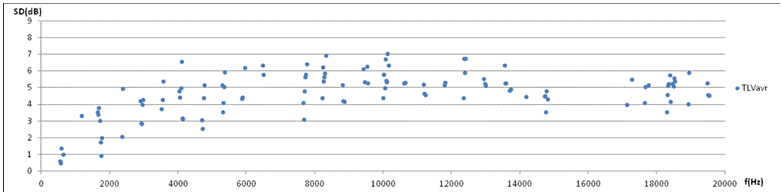
17a. Temporal level variation TLV in terms of standard deviation of M=10 periods (t=50ms) from 14700ms, average of five directions plotted against frequency. TLV rises steeply above the fundamental. Above 5300Hz (9th harmonic) the TLV appears to fluctuate around an average of 5.2dB. |
||||||||||||||||||||||||||||||||||||||||||||||||||||||||
|
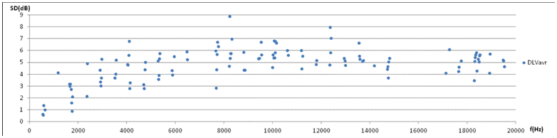
17b. Directional level variation DLV in terms of standard deviation of N=5 directions, average of 10 periods (50ms) from 14700ms plotted against frequency. DLV rises steeply above the fundamental. Above 5300Hz (9th harmonic) the DLV appears to fluctuate around an average of 5.4dB. |
||||||||||||||||||||||||||||||||||||||||||||||||||||||||
|
|
||||||||||||||||||||||||||||||||||||||||||||||||||||||||
|
|
||||||||||||||||||||||||||||||||||||||||||||||||||||||||
|
17e. Correlation (Pearsons r2) between the 5 channels, average of the10 pertubations 1-2,1-3,1-4,1-5,2-3,2-4,2-5,3-4,3-5,4-5., plotted against frequency. Average over the whole frequency range is low, r=0.18, with slightly increasing values towards 0Hz, however less prominent frequency dependency than the cross-correlation between channels seen in the vibrato style D5 note in (7e). |
||||||||||||||||||||||||||||||||||||||||||||||||||||||||
|
18. Peak radiation. The peak direction is the direction in which the radiated intensity is the strongest. The plot displays probability of the instant peak direction being equal to long-term average peak direction. On a probability scale from 0 to 100%, 100% would mean that peak radiation was constantly equal to long-term average peak direction, and 20% would indicate that peak direction is perfectly random. Average probability over the whole frequency range is 25%, meaning that peak direction is relatively close to random over the 10 analyzed instants. In this context, an ”instant” is a time window of 50ms. |
||||||||||||||||||||||||||||||||||||||||||||||||||||||||
|
19a. Comment: The set of TLV above 5300Hz is not statistically significant (p=0.05) from the set of DLV in the same frequency range. TLV and DLV is highly correlated, r=0.95. DLV correlates higher with the whole data set, r=0.97. TLV average 5.2dB is just significantly (p=0.05) different from whole data set (M*N) average 5.5dB, but they correlate highly at r=0.96. Results from the study of the vibrato-free D5 note part starting at 14700ms (steps 11-18), do not differ significantly from the results from the study of the vibrato part of the same note (steps 1 to 8). 19b. Conclusion: The vibrato sequence and the vibrato-free sequence at note D5 both show the same general features of dynamic directivity. Both the temporal and directional level variations are random outcomes of a stochastic prosess at higher frequency, however tending towards zero variation as frequency approaches 0Hz. Levels fluctuate over time and over directions, centered around a floating average which for longer periods of time assumably will approach the long-term average spectrum measured in each direction (each channel), demonstrated for channel 1 by the bold curve in Fig 4 and Fig 14. 19c. Further work: In order to investigate dynamic directivity in a music instrument very different from a violin, an oboe playing the 1st oboe part in the same Mozart piece as the violin above, is chosen. |
||||||||||||||||||||||||||||||||||||||||||||||||||||||||
|
|
||||||||||||||||||||||||||||||||||||||||||||||||||||||||
|
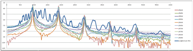
21. Oboe. Wave-form (dB) versus time, anechoic recording of Oboe 1 in front of player (ch1), first 1 min and 50 sec of Mozart Symphony No 40, G-minor. Compared to the 1st violin (fig 1 and 11), the oboe plays fewer notes and plays approximately half of the time. Fewer notes usually means that the long-term spectrum (20 above) will be less continous, with more peaks and dips. The window chosen for detailed analysis is marked at 25400ms. |
||||||||||||||||||||||||||||||||||||||||||||||||||||||||
|
22. Spectrogram corresponding to the wave-form in Fig 21. The grey-marked 500ms period at 25400ms is subject to more detailed analysis below . |
||||||||||||||||||||||||||||||||||||||||||||||||||||||||
|
|
||||||||||||||||||||||||||||||||||||||||||||||||||||||||
|
24. Spectrum of ch 1, long-term spectrum (bold curve) and ten 50ms-window spectra between 25400ms and 25900ms; FFT size 2048. The upper harmonics are smeared out in frequency due to the slight vibrato, see Fig 3. Only the first 5 harmonics have sufficient level to be qualified for the following directionality analysis. The oboe has a lower number of strong harmonics than the violin. |
||||||||||||||||||||||||||||||||||||||||||||||||||||||||
|
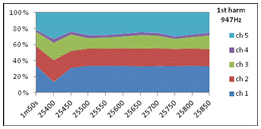
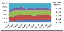
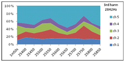
25. Dynamic directivity at first five harmonics of A#5. Compared to (5) and (15), less variations are seen in 1st and 2nd harmonic of the oboe than in the violin. However, a general tendency of increasing level variations in higher harmonics is seen also in the oboe. |
||||||||||||||||||||||||||||||||||||||||||||||||||||||||
|
26a. Statistics corresponding to 1st and 2nd harmonic of A#5, upper diagrams in Fig 25. Temporal level variation TLV in each of the five direction (channel) in terms of standard deviation of intensity levels in M=10 periods of 50ms length. A plot of the whole frequency range is presented in Fig 17 below. |
||||||||||||||||||||||||||||||||||||||||||||||||||||||||
|
26b. Statistics from Fig 25. Directional level variation DLV in each of the ten 50ms periods, in terms of standard deviation of intensity levels in five directions (channels). Longterm DLV in leftmost column for comparison. A plot of the whole frequency range is presented in Fig 27 below. 26a-26b comparison: Level variation over instants are practically equal to level variations over directions. In contrast to violin results (compare with 6 and 16 above), variations in 1st harmonic is of the same size as variations in 2nd harmonic. 26c. Level variation over the whole data of size M*N=10*5=50 exhibits a standard deviation of 0.6dB in the narrowband centered at 947 Hz, while 0.7dB at 1895Hz. Level variation of all harmonic components are plotted in Fig 27 below. |
||||||||||||||||||||||||||||||||||||||||||||||||||||||||
|
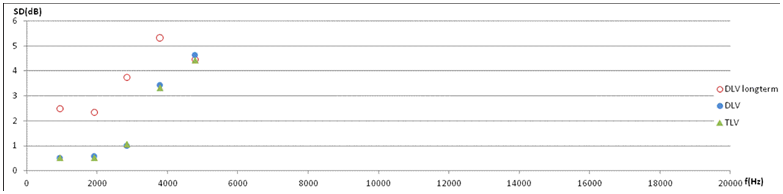
27. Level variations measured in Oboe1 at the lower 5 harmonics of A#5 note plotted against frequency. 1st and 2nd harmonic plots are the values in tables 26a-b. Temporal level variation TLV and directional level variation DLV are practically equal in all five harmonics. Long-term DLV i noteably higher than TLV and DLV in the lower first four harmonics, but in the 5th harmonic, all three level variation parameters are practically equal at 4.5-4.7dB. Compared to violin results (7a-c and 17a-c), TLV and DLV in the oboe show much lower values in harmonics below 4kHz, while the difference in long-term long-term DLV is more like an octave transpose: The rise in long-term DLV from 2dB to 5dB is seen in the region 0-4kHz (harmonics 1 to 4) in the Oboe, while the same rise is seen in 0-2kHz (harmonics 1-3) in the Violin. Another major difference between Oboe results and Violin results is obviously the lack of harmonic energy above 5kHz in the oboe, as is clearly demonstrated in the plot above. |
||||||||||||||||||||||||||||||||||||||||||||||||||||||||
|
28. Window Length Discussion and Test. In steps 0 and 20 above, the analysis windows are 1m50s, i.e. Long-term analysis window. All other analysis windows are 50ms. One suspects that as analysis windows get longer, level differenses over time are integrated, level variations are averaged out, and thus TLV is expected to become smaller. However DLV might not change in the same way. In order to discuss the significance of analysis window length, an extensive test program has been performed, repeating the procedure 0-19 for window lengths 50ms, 100ms, 200ms, 400ms, 10s and 1m 50s. Results are given in the table below. ”sd” is the standard deviation of all channeles and periods (data size M*N). ”X-corr” is the cross-correlation between all possible channel pairs 1-2, 1-3, 1-4, 1-5, 2-3, .. etc. ”R2” is Pearson correlation r2 between directivity pattern of window and long-term directivity pattern. ”peak prob” is the probability of finding peak direction of the window equal to the long-term peak direction. Comment: TLV decrease with increasing window length up to 400ms. TLV may seem to approach DLV as window length decreases, leaving the question: Will TLV and DLV approach the same limit as window length approaches zero? Inter-channel correlation ”X-corr” increases with window lengths, and so does ”R2” and ”peak prob”.
|
||||||||||||||||||||||||||||||||||||||||||||||||||||||||
|
To be continued First published 09.12.2011, latest change 16.01.2012 Go to www.akutek.info main page Go to article site index page |